Vector Addition: Graphical Methods

Vector addition is the quiet engine behind almost every two-dimensional motion problem a learner will ever meet. A boat crossing a river, a plane drifting in crosswind, a hiker following two legs of a trail — each scenario resolves into the same geometric question: how do two directed quantities combine into one? This lesson answers that question with pencil, ruler, and protractor rather than algebra, because seeing the geometry first makes the later analytical machinery feel inevitable rather than arbitrary.

Building directly on the distinction between scalars and vectors established in the previous lesson, the material here treats arrows as objects that can be moved, chained, and completed into parallelograms. The head-to-tail rule and the parallelogram method are presented as two views of one underlying truth, and the commutative property emerges from the drawings themselves. By the end, learners will construct resultants by hand, estimate their magnitudes and directions, and understand why the order of addition never matters.

This is deliberately a graphical lesson. Numbers arrive in the next session, when components and trigonometry take over. For now, the goal is spatial intuition: a felt sense of how direction and magnitude interact when vectors are combined. That intuition will act as a sanity check for every calculation that follows in the course, from projectile trajectories to the centripetal acceleration of uniform circular motion.

Why Graphical Addition Comes First

Before any formula appears, physics asks learners to see. Graphical vector addition trains the eye to judge whether a computed answer is plausible, catching sign errors and swapped components that pure algebra can hide. A resultant drawn to scale either points roughly where intuition expects or it does not, and that visual verdict is often faster than rechecking arithmetic.

The approach also respects how the concept historically developed. Navigators, surveyors, and military engineers combined displacements with compass and chain long before coordinate geometry formalized the operation. Reproducing their method connects abstract notation to physical practice, and it gives beginners a concrete anchor when symbolic manipulation later becomes dense.

Arrows as Displacements

A vector is drawn as a straight arrow whose length encodes magnitude and whose orientation encodes direction. In graphical work, the scale is chosen freely — one centimetre per ten newtons, say — and every vector in a given diagram must obey that same scale or the drawing lies. Consistency of scale is the single most important discipline in this method.

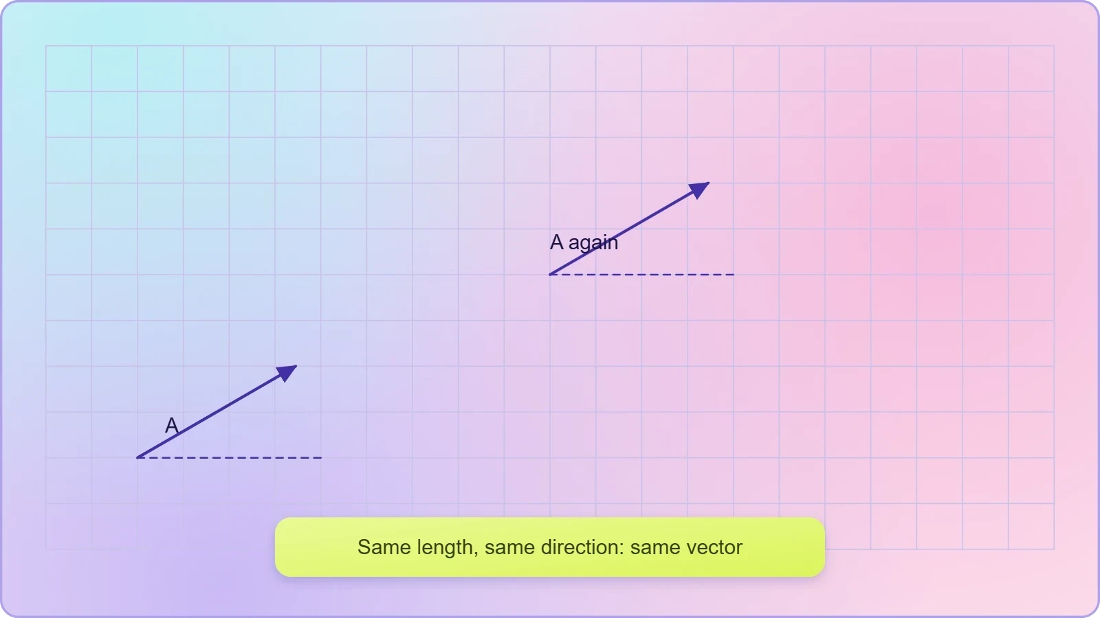
Position within the plane is irrelevant; only length and orientation carry meaning. A vector may be slid anywhere on the page without changing it, a property called invariance under translation. This freedom is precisely what permits the head-to-tail construction, because it lets us relocate the second arrow so its tail meets the first arrow's head.

Setting Up a Scale Drawing

Practical construction begins with a sharp pencil, a ruler, a protractor, and graph paper. Choose a scale that keeps the largest vector within the page while preserving resolution for the smallest, then record the scale beside the diagram. Angles are measured from a stated reference direction, conventionally the positive x-axis, and marked carefully.

Accuracy matters more than neatness, though both help. A one-degree protractor error over a long chain of vectors compounds into a visibly wrong resultant, which is itself a useful lesson about experimental uncertainty. Learners should annotate every arrow with its magnitude and angle so the drawing can be audited later.

The Head-to-Tail Rule in Practice

The head-to-tail rule is the workhorse of graphical addition. Place the tail of the second vector at the head of the first, then draw the resultant from the original tail to the final head. The procedure extends to any number of vectors simply by continuing the chain, and the closing arrow always represents the total displacement.

This construction mirrors physical experience directly. Walking three blocks east and then four blocks north leaves you five blocks from where you started, and the diagonal of the drawing is that displacement. The rule converts a sequence of separate motions into a single equivalent motion, which is exactly what "resultant" means.

Constructing a Two-Vector Resultant

Draw the first vector to scale from a chosen origin. At its tip, draw the second vector at the correct angle relative to a parallel reference line, not relative to the first arrow's direction unless the problem specifies it. Then connect the origin to the second arrow's tip with a third arrow, the resultant.

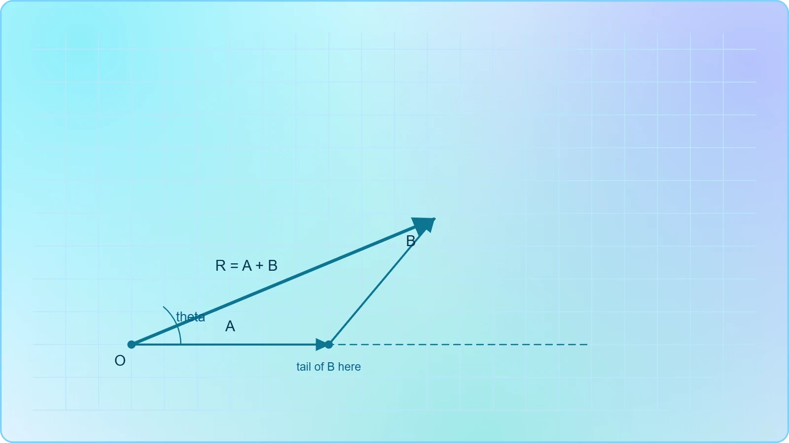
Measure the resultant's length and convert back through the scale to obtain its magnitude. Measure its angle with the protractor against the same reference used throughout. Record both values with sensible significant figures, acknowledging that a drawing rarely justifies more than two or three digits of precision.

Chaining Three or More Vectors

Polygons of vectors follow the same logic without modification. Add the third vector at the head of the second, the fourth at the head of the third, and so on; the resultant closes the figure from first tail to last head. Order of placement is arbitrary, and the final closing arrow is identical regardless.

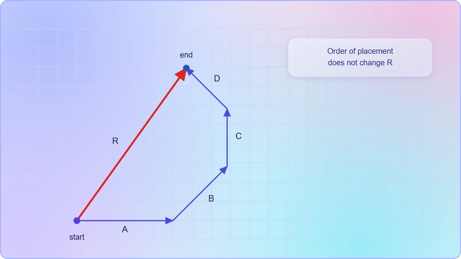
When the chain returns to its starting point, the resultant is zero and the vectors are in equilibrium. This closed-polygon condition is the graphical statement of balanced forces, and it reappears throughout mechanics whenever an object sits at rest under several concurrent pulls. Recognising a closed polygon is a quick equilibrium test.

The Parallelogram Method and Its Geometry

An alternative construction places both vectors tail-to-tail at a common origin and completes the parallelogram they span. The diagonal drawn from that shared origin is the resultant. This method is especially natural when two forces act on a single point, because both arrows then genuinely share their point of application.

The parallelogram and head-to-tail approaches are geometrically identical, merely drawn from different starting conventions. Sliding one arrow to the head of the other converts one picture into the other. Understanding this equivalence frees learners from memorising two separate procedures when only one idea is at work.

Drawing the Parallelogram

From a common origin, draw both vectors at their true angles. Construct a line through the head of the first vector parallel to the second, and a line through the head of the second parallel to the first. Their intersection is the fourth vertex, and the diagonal from the origin to that vertex is the resultant.

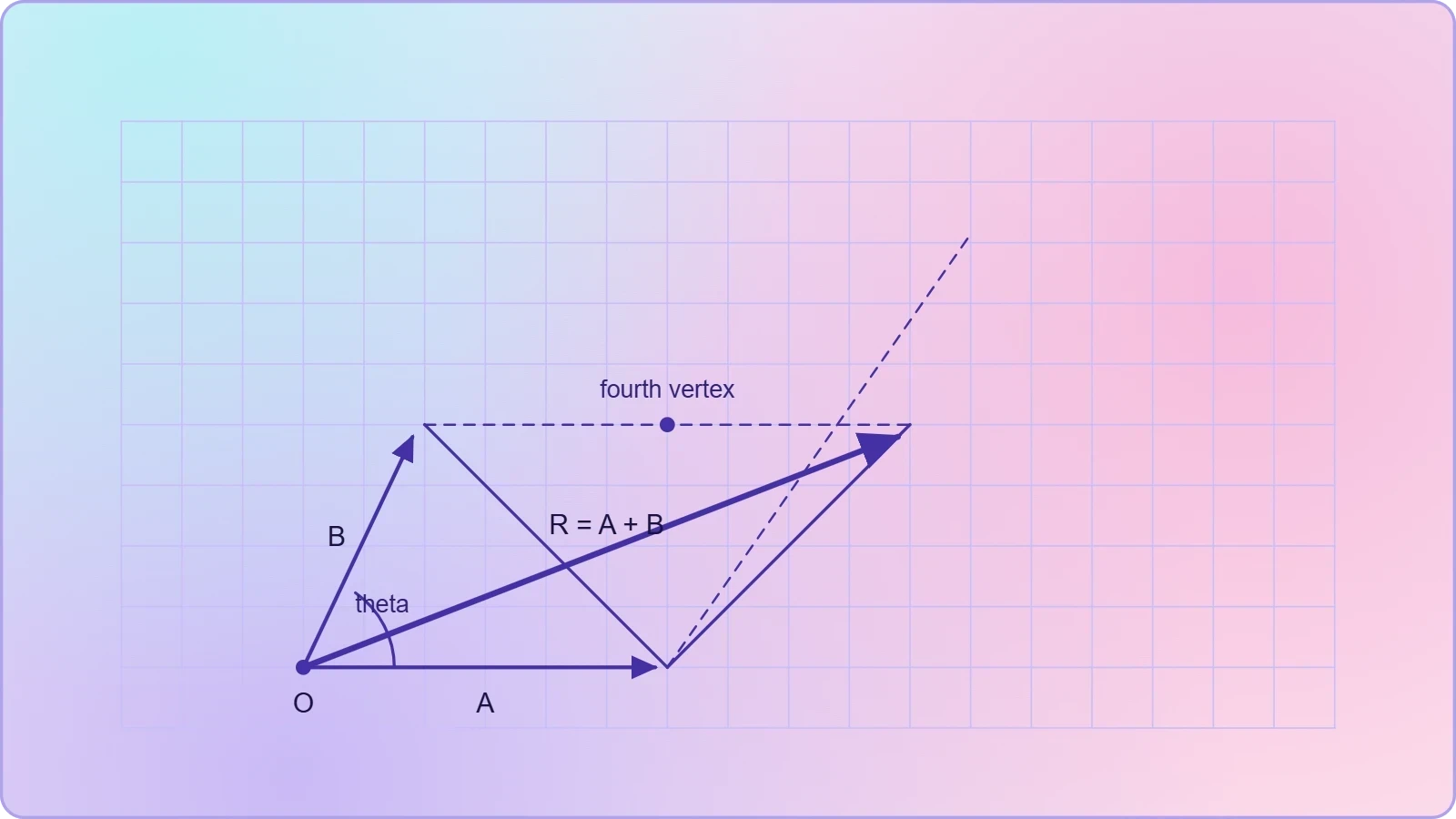
Parallel lines are easiest to produce with a set square or by counting grid squares on graph paper. The diagonal's length and angle are then measured exactly as in the head-to-tail method. The construction is symmetric in the two vectors, which already hints at the commutative law.

Reading the Diagonal

The diagonal of the parallelogram represents the vector sum, while the other diagonal represents the vector difference. That second diagonal, drawn from the head of one vector to the head of the other, points along the direction of subtraction. Recognising both diagonals gives a single diagram double duty.

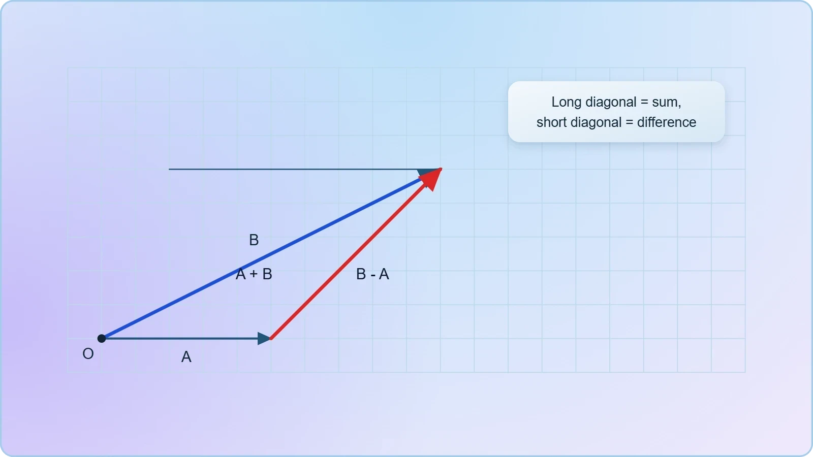
For perpendicular vectors, the parallelogram becomes a rectangle and the diagonal's length follows the Pythagorean relation. This special case is worth drawing repeatedly, because it previews the component method arriving in the next lesson and makes the transition to algebra feel like a natural extension rather than a new topic.

Commutativity, Associativity, and the Zero Vector

Graphical addition makes the algebraic laws visible rather than asserted. Reversing the order of two vectors simply relabels the same parallelogram, so the resultant is unchanged. This is commutativity, and the drawing proves it in a single glance without a line of algebra.

Associativity appears when three vectors are chained: grouping the first two and adding the third yields the same closing arrow as grouping the last two first. The polygon is identical either way. These properties are not decorative; they license the reordering and regrouping that later analytical work depends upon.

Order Does Not Matter

Because the parallelogram is symmetric under swapping its adjacent sides, ##\vec{A} + \vec{B} = \vec{B} + \vec{A}## holds for every pair of vectors. Learners should verify this by drawing both orders on separate sheets and comparing the closing arrows. The exercise takes minutes and permanently settles the question.

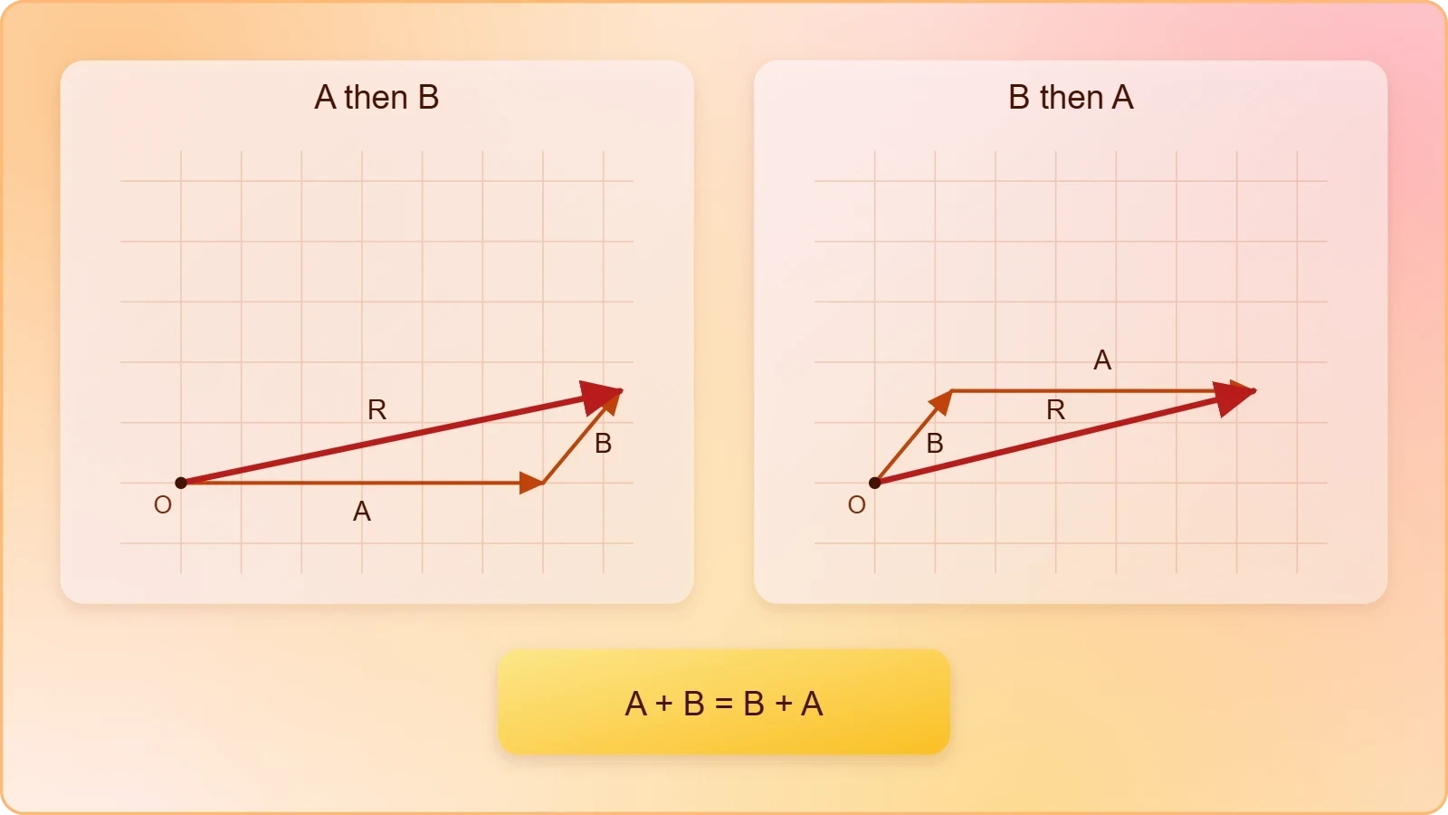
Commutativity extends to any finite collection of vectors, so a long chain may be rearranged freely before drawing. This flexibility is practically useful when some vectors are easier to place first, and it underpins the component method, where x and y contributions are summed independently in whatever order suits the solver.

The Resultant of Opposing Vectors

When two vectors point in exactly opposite directions, the parallelogram collapses into a line segment. The resultant magnitude is the absolute difference of the two magnitudes, directed along the larger vector. This degenerate case is the graphical origin of vector subtraction and deserves explicit attention.

If the opposing vectors are equal in magnitude, the resultant vanishes entirely. The zero vector has no defined direction and is represented by a point rather than an arrow. Encountering it graphically prepares learners for equilibrium problems, where the sum of all forces on a stationary body must equal zero.

Worked Examples with Scale Drawings

Concrete problems cement the method. Consider a hiker who walks 4.0 km east, then 3.0 km north. Choosing one centimetre per kilometre, the drawing produces a right triangle whose diagonal measures five centimetres, so the resultant displacement is 5.0 km at roughly 37 degrees north of east.

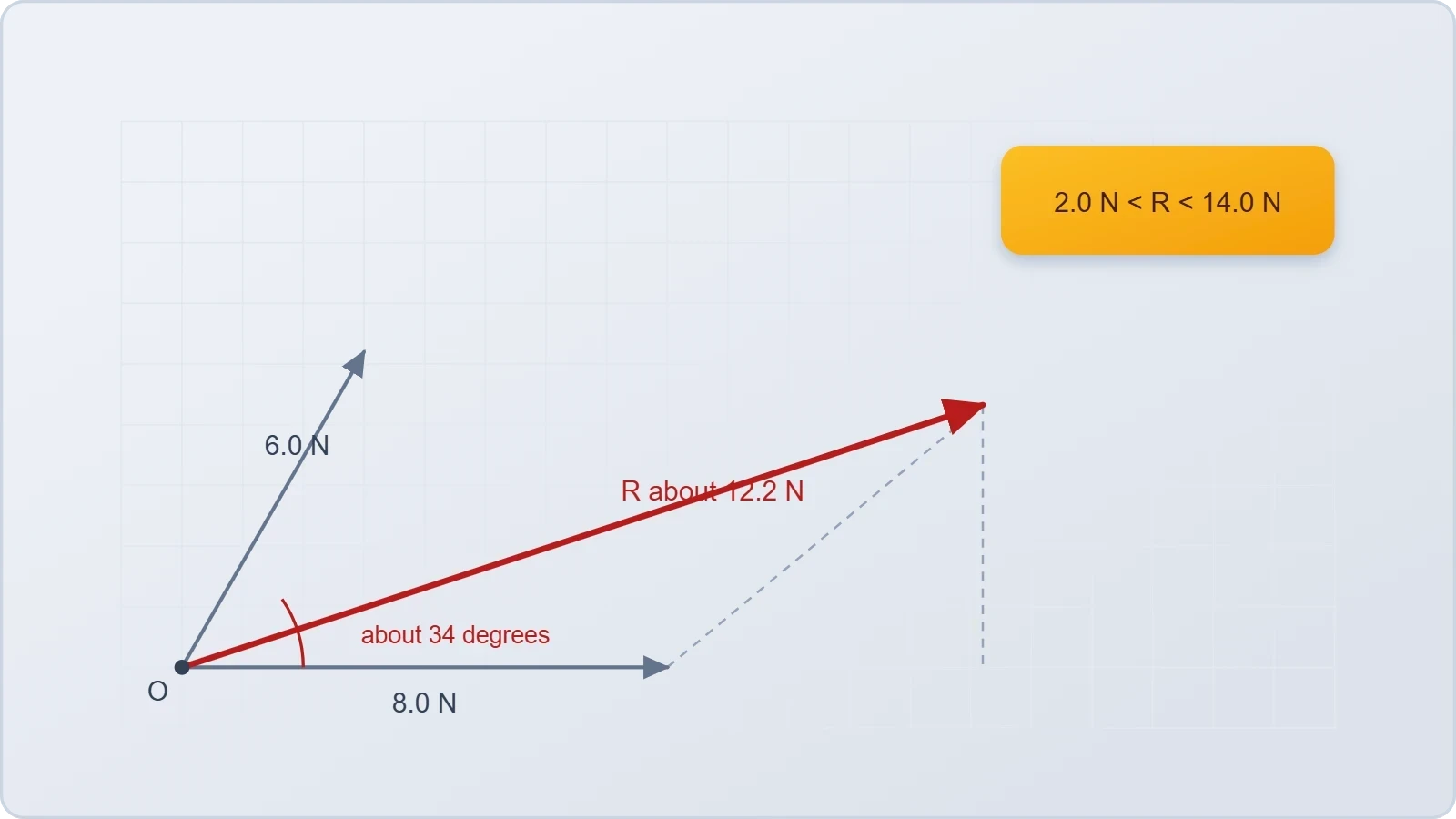
Now consider two forces of 6.0 N and 8.0 N acting at 60 degrees to each other. The parallelogram diagonal measures about 12.2 N on the chosen scale, and the measured angle falls near 34 degrees from the larger force. The drawing supplies both answers before any trigonometry is invoked.

A Displacement Problem

For the hiker, the head-to-tail chain is trivial: two perpendicular arrows, one closing diagonal. The scale conversion is direct, and the protractor reading confirms the angle. Learners should repeat the construction at a different scale to confirm the resultant is scale-invariant, as it must be.

Variations deepen understanding. Reverse the order of the two legs and the resultant is identical, demonstrating commutativity physically. Replace the second leg with a southwest walk and the diagonal shortens, showing how direction, not just distance travelled, governs the final displacement.

A Force Problem

Forces acting at a point suit the parallelogram method, since both arrows share their origin naturally. Draw 6.0 N and 8.0 N at 60 degrees, complete the parallelogram, and measure the diagonal. The result near 12.2 N sits between the arithmetic sum of 14 N and the difference of 2 N, as it always must.

This bracketing rule is a powerful self-check: the magnitude of any resultant lies between the difference and the sum of the individual magnitudes. If a drawing or later calculation violates that bound, an error has occurred. Learners should apply the test routinely before trusting any answer.

Common Errors and How to Avoid Them

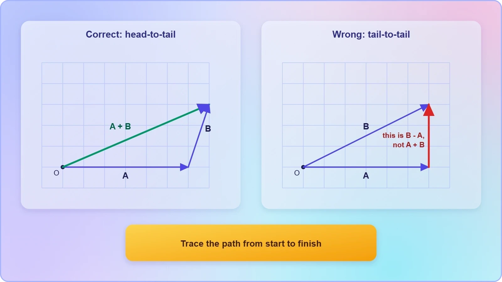
The most frequent mistake is attaching the second vector tail-to-tail and then drawing a diagonal from the wrong point. That construction yields the difference, not the sum. Learners should always trace the path physically: start at the origin, follow the first arrow, continue along the second, and close from start to finish.

A second error is measuring the second vector's angle relative to the first arrow rather than to the fixed reference axis. Angles in vector problems are almost always given against a common frame, and misreading them skews the entire drawing. Marking the reference direction prominently on the page prevents this.

Scale and Measurement Pitfalls

Inconsistent scale, blunt pencils, and protractors read from the wrong baseline all corrupt results. Use a sharp 0.5 mm pencil, align the protractor carefully, and double-check every length against the ruler before committing. Small drafting errors accumulate quickly in longer chains and can flip a resultant's apparent direction.

Overstating precision is equally damaging. A drawing measured to the nearest millimetre on a scale of one centimetre per unit justifies at most two significant figures. Reporting 12.237 N from a protractor sketch misrepresents the method's accuracy and invites false confidence in later numerical work.

Interpreting the Resultant Correctly

Remember that the resultant replaces the original vectors entirely; it is not an additional force. In equilibrium problems, the resultant of all applied forces is zero, and any single force is balanced by the sum of the others. Confusing the resultant with an extra applied vector leads to double counting.

Direction deserves equal care. A magnitude without a stated angle is incomplete, since the same length can point anywhere on the compass. Always report the resultant as a magnitude together with an angle measured from a clearly identified reference, and state the sense of rotation explicitly.

From Drawings to Components: Preparing for Lesson Four

Graphical methods build intuition, but they are slow and imprecise for routine calculation. The next lesson replaces ruler and protractor with trigonometry, resolving each vector into perpendicular components and summing them algebraically. The drawings remain valuable as verification, yet the arithmetic takes over the heavy lifting.

Everything learned here transfers directly. The parallelogram's diagonal becomes the hypotenuse of a right triangle whose legs are the components. The head-to-tail chain becomes a column of x-terms and a column of y-terms. Recognising this continuity turns the analytical method into a refinement rather than a replacement.

What Carries Forward

The commutative and associative laws survive unchanged in component form, which is why components may be summed in any convenient order. The bracketing rule persists as a check on computed magnitudes. The zero-vector condition reappears as the requirement that both component sums vanish simultaneously for equilibrium.

Learners who have drawn many polygons will find the component method almost obvious: it is the same addition, executed along two perpendicular axes instead of on open paper. That conceptual bridge is the chief purpose of this lesson, and it should be crossed deliberately rather than skipped.

A Brief Programming Check

Computers perform vector addition by summing components, but a short script can also verify a graphical result. The snippet below adds two planar vectors and reports the resultant magnitude and direction, mirroring what a careful drawing would show.

import math

def add_vectors(v1, v2):
    rx = v1[0] + v2[0]
    ry = v1[1] + v2[1]
    magnitude = math.hypot(rx, ry)
    angle = math.degrees(math.atan2(ry, rx))
    return (rx, ry), magnitude, angle

resultant, mag, ang = add_vectors((4.0, 0.0), (0.0, 3.0))
print(resultant, round(mag, 2), round(ang, 1))

Running this with the hiker's displacements returns a magnitude of 5.0 and an angle near 36.9 degrees, matching the scale drawing within measurement tolerance. Such cross-checks build confidence that the geometric and algebraic pictures describe one and the same operation.