Problem-Solving Strategies for 2D Motion

Two-dimensional motion problems intimidate learners not because the physics is exotic, but because the bookkeeping is unforgiving. A single misplaced sign, a forgotten component, or an unchecked unit can quietly corrupt an otherwise elegant solution. This lesson treats problem-solving as a discipline in its own right, offering a repeatable method that transforms messy scenarios into orderly, verifiable calculations.

Building directly on the vector fluency established in the previous lesson, we now convert that vocabulary into a working procedure. You will learn how to dissect a problem statement, isolate horizontal and vertical behaviour, select the right kinematic relations, and audit your final answer against physical intuition. Each stage is illustrated with worked reasoning rather than memorised templates.

The approach is deliberately systematic: read, sketch, decompose, solve, and verify. Master this loop and projectile questions, circular-motion puzzles, and relative-velocity riddles all begin to feel like variations on a single theme. The goal is not speed but reliability, because a method you trust is worth more than a formula you half-remember.

The Anatomy of a Two-Dimensional Motion Problem

Every well-posed problem in the plane contains the same skeleton: an object, an initial state, a set of forces or accelerations, and a question about a later state. Recognising this skeleton early lets you map the given data onto the kinematic variables before any algebra begins. The discipline lies in separating what is stated from what is implied.

Reading the Problem Statement Like a Physicist

Begin by underlining every numerical value and tagging it with a symbol and a direction. A launch speed of ##20\ \text{m/s}## at ##30^\circ## above the horizontal is not one datum but two components waiting to be extracted. Ambiguities such as "returns to the ground" or "just clears the wall" encode boundary conditions that constrain the equations.

Sketching follows immediately, because a diagram exposes relationships that prose conceals. Mark the coordinate axes, the initial velocity vector, and any known positions. A clean sketch frequently reveals that the problem is simpler than the wording suggests, or that a hidden symmetry halves the required work.

Separating Knowns, Unknowns, and Constraints

List the known quantities in one column and the unknowns in another, then note the constraints that link them. In projectile problems the horizontal and vertical motions share only the time variable, which becomes the bridge between the two component equations. Identifying that bridge early prevents circular reasoning later.

Constraints also include physical limits: the ground, a ceiling, a target radius, or a maximum tension. Treating these as equations rather than afterthoughts keeps the solution honest. When a constraint is violated, the mathematics is telling you the scenario is impossible, not that the algebra failed.

Decomposing Motion into Independent Components

The central insight of planar kinematics is that perpendicular directions do not interfere. Horizontal velocity persists unchanged while gravity acts vertically, and vertical motion proceeds as though the horizontal component never existed. This independence is what makes component methods so powerful and so easy to misapply.

Choosing Axes That Simplify the Algebra

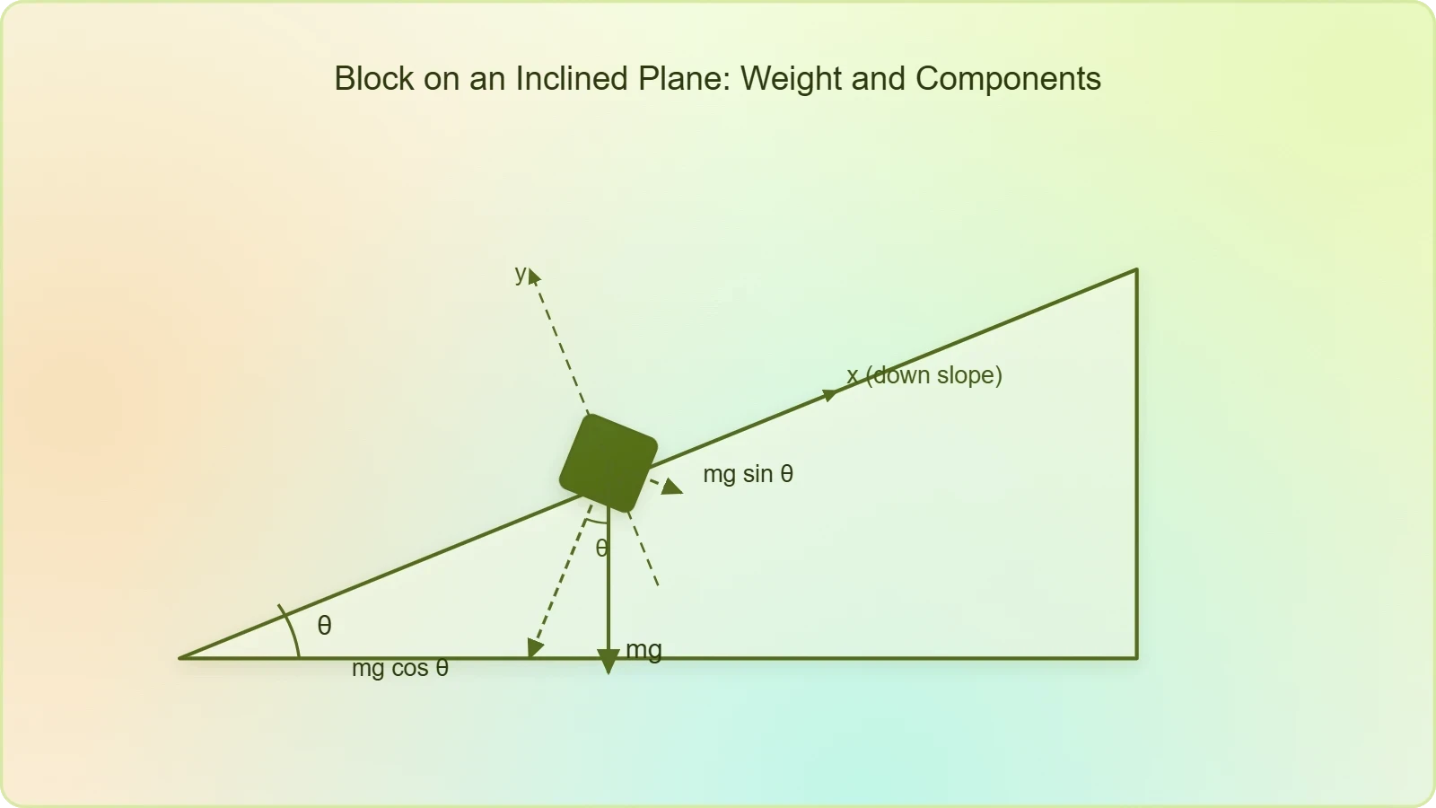
Conventional axes align horizontal with the x-direction and vertical with y, but the choice is yours to optimise. On an inclined plane, tilting the axes so one runs along the slope converts a two-acceleration problem into a single-acceleration one. Good axis selection is a strategic decision, not a formality.

Once axes are fixed, resolve every vector into those directions using ##v_x = v\cos\theta## and ##v_y = v\sin\theta##. Keep the angle measured consistently from the same reference, and record signs according to your chosen positive directions. Inconsistent conventions are the most common source of silent errors.

Applying Component Equations with Shared Time

With components in hand, write the kinematic relations separately for each axis. The horizontal equation typically reads ##x = v_x t##, while the vertical follows ##y = v_y t - \tfrac{1}{2}gt^2##. Time appears in both, and that shared variable is the hinge on which the solution turns.

Solve the simpler equation for time first, then substitute into the other. This ordering avoids quadratic complications whenever the horizontal relation is linear. When both equations are quadratic in time, expect two mathematical roots and interpret each physically before discarding one.

Selecting the Right Equation for the Question Asked

Kinematics offers five variables and several relations linking them, and the art lies in choosing the relation that contains exactly one unknown. Count the variables you know, identify the one you need, and pick the equation that connects them without dragging in irrelevant quantities. This single habit eliminates most wasted algebra.

Matching Variables to Equations

If time is absent from both the data and the question, the time-free relation is your instrument. If displacement is unknown but time is given, the velocity relation suffices. Treating the equation set as a lookup table keyed on missing variables turns selection into a mechanical, error-resistant step.

When two unknowns remain, you need two equations, and the shared time variable usually supplies the second. Write both relations before solving either, so the system is visible as a whole. Solving one equation prematurely often hides the cleaner path through the problem.

Handling Relative Velocity and Circular Cases

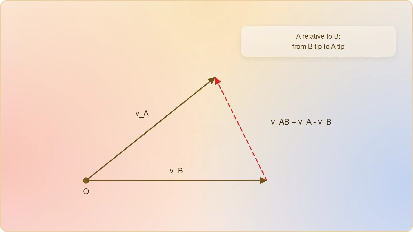
Relative-velocity problems obey vector subtraction: the velocity of A relative to B is ##\vec{v}_{AB} = \vec{v}_A - \vec{v}_B##. Draw the triangle or parallelogram before computing, because the geometry usually reveals whether the answer is a sum, a difference, or a perpendicular combination.

Uniform circular motion replaces linear acceleration with centripetal acceleration directed toward the centre, of magnitude ##a_c = v^2/r##. Here the strategy shifts: resolve forces along radial and tangential directions rather than horizontal and vertical, and let the geometry of the circle define your axes.

Worked Reasoning: A Projectile and a Turning Vehicle

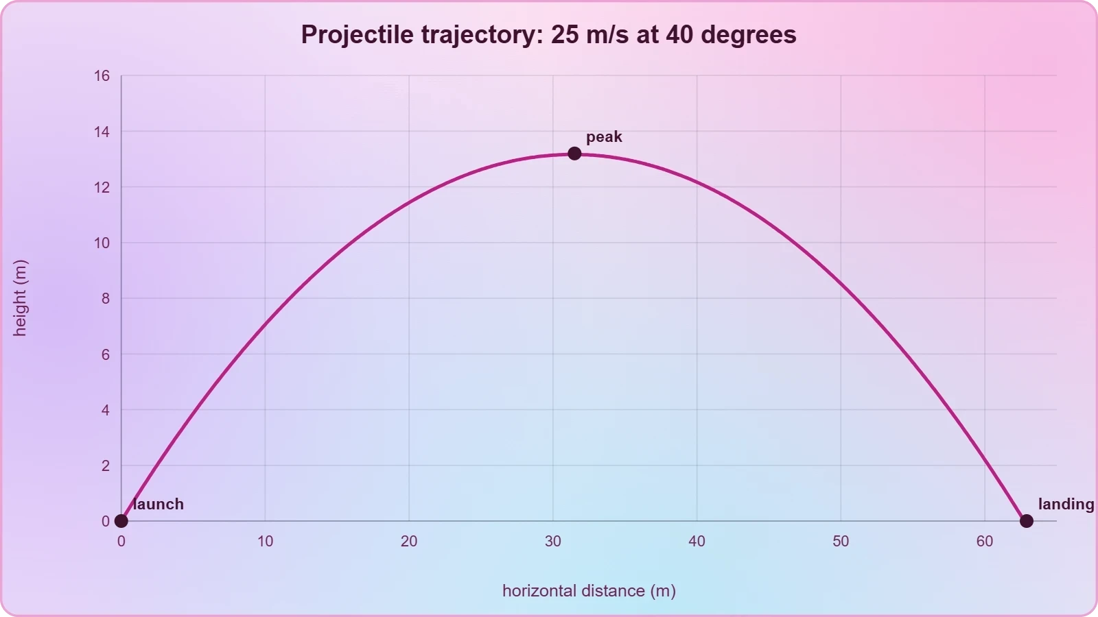
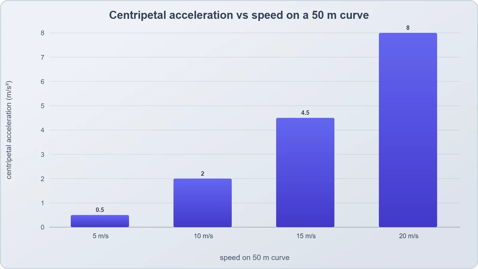
Abstract strategy becomes credible only when applied. Consider a ball launched at ##25\ \text{m/s}## and ##40^\circ## above horizontal from level ground, and separately a car rounding a flat curve of radius ##50\ \text{m}## at ##15\ \text{m/s}##. Both yield to the same five-step loop, though their physics differs.

Projectile Flight from Launch to Landing

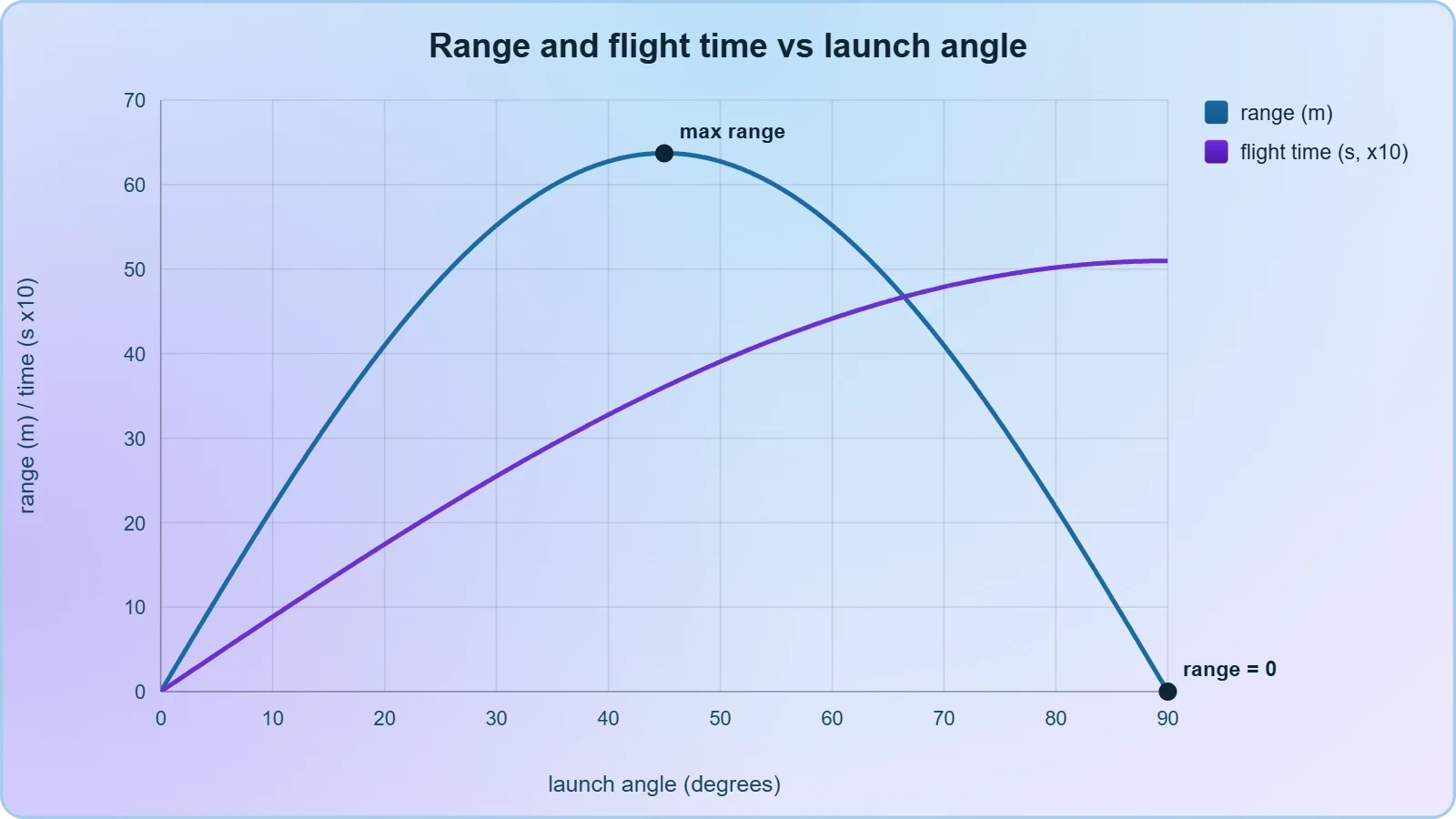
Resolve the launch velocity into ##v_x \approx 19.2\ \text{m/s}## and ##v_y \approx 16.1\ \text{m/s}##. Setting vertical displacement to zero gives the flight time ##t = 2v_y/g \approx 3.28\ \text{s}##, from which the horizontal range follows as roughly ##63\ \text{m}##.

Check the result against intuition: a launch angle near ##45^\circ## should maximise range for a given speed, and ##40^\circ## sits close to that optimum. The peak height, ##v_y^2/2g \approx 13.2\ \text{m}##, is modest and consistent with a three-second flight. Every number coheres.

Circular Motion and Required Friction

For the turning car, the centripetal requirement is ##a_c = v^2/r = 225/50 = 4.5\ \text{m/s}^2##. Static friction must supply this acceleration, so the minimum coefficient satisfies ##\mu_s g \ge 4.5##, giving ##\mu_s \approx 0.46##. A wet road with lower friction would force a slower speed.

Notice how the strategy transfers: identify the constraint, express it as an equation, solve for the unknown, then interrogate the answer. The projectile used geometry and time; the car used force balance and radial acceleration. The procedural skeleton remained identical throughout both cases.

Verifying Answers Through Units, Signs, and Limits

A computed number is a hypothesis until it survives scrutiny. Verification is not optional polish; it is the step that separates a confident solution from a lucky one. Three checks catch nearly every error: dimensional consistency, sign plausibility, and behaviour in limiting cases.

Dimensional Analysis and Order-of-Magnitude Checks

Every term in an equation must carry the same units, so a quick dimensional audit exposes mismatched expressions instantly. If a distance is equated to a velocity, something has gone wrong upstream. This check costs seconds and routinely rescues entire solutions from silent corruption.

Order-of-magnitude reasoning complements the audit. A thrown ball should travel metres, not kilometres; a car on a dry road should manage a friction coefficient below unity. When a result lands far outside the expected band, revisit the inputs before trusting the output.

Sign Conventions and Physical Plausibility

Signs carry physical meaning, and a negative time or a negative speed signals a modelling error rather than an exotic discovery. Confirm that upward is consistently positive or consistently negative, and that every vector's direction matches the story the problem tells.

Finally, test limiting behaviour: as the launch angle approaches ##90^\circ##, range should shrink toward zero while flight time grows. If your general expression fails these extremes, the algebra contains a flaw. Limits are the cheapest stress test available to any student.

Building a Personal Problem-Solving Routine

Strategy becomes skill only through repetition, and repetition is most effective when structured. Adopt a fixed sequence, apply it to every problem for a fortnight, and the loop will become automatic. Consistency, not cleverness, is what separates reliable solvers from anxious ones.

From Worked Examples to Independent Practice

Study worked solutions actively by covering the algebra and predicting each next step. When your prediction diverges from the printed line, you have located a genuine gap in understanding. This technique converts passive reading into targeted diagnosis and accelerates improvement far beyond re-reading notes.

Then attempt fresh problems under mild time pressure, narrating your reasoning aloud. Verbalising the five-step loop exposes fuzzy assumptions that silent calculation conceals. Keep an error log categorised by failure type, and review it weekly to spot recurring weaknesses before they harden into habits.

Preparing for Air Resistance and Beyond

The next lesson relaxes our idealisation by introducing air resistance qualitatively, and your routine must adapt rather than break. Drag makes trajectories asymmetric and ranges shorter, so verification shifts toward qualitative reasoning about trends rather than exact numerical equality.

Anticipate that the component method survives, but the equations no longer solve cleanly. Recognising when a model's assumptions fail is itself a problem-solving skill, and it will serve you well beyond this course. The method you have built here is a foundation, not a cage.

A short script can automate the arithmetic while you concentrate on reasoning. The function below resolves a launch velocity, computes flight time and range, and prints a verification summary for a level-ground projectile.

import math

def projectile_summary(speed, angle_deg, g=9.8):
    theta = math.radians(angle_deg)
    vx = speed * math.cos(theta)
    vy = speed * math.sin(theta)
    flight_time = 2 * vy / g
    peak_height = vy**2 / (2 * g)
    rng = vx * flight_time
    return {
        "vx": round(vx, 2),
        "vy": round(vy, 2),
        "time": round(flight_time, 2),
        "height": round(peak_height, 2),
        "range": round(rng, 2),
    }

result = projectile_summary(25, 40)
print(result)
assert result["range"] > 0, "Range must be positive"
assert result["time"] < 10, "Flight time implausible for a hand throw"

The assertions embody the verification habit: they encode physical expectations as executable checks. Run the script, compare its output with your hand calculation, and treat any disagreement as a prompt to audit both. Automation should confirm understanding, never replace it.