Graphical Analysis of Motion in a Plane

Graphical analysis of motion in a plane transforms abstract vector equations into visual stories that the eye can read at a glance. When a particle moves across a flat surface, its horizontal and vertical behaviours unfold simultaneously, and plotting each component against time reveals patterns that raw numbers often conceal. This lesson builds directly on the synthesis work of the previous session, where position, velocity, and acceleration vectors were combined into a single coherent description of two-dimensional motion.

Rather than treating graphs as decorative illustrations, we will treat them as analytical instruments. A position-time curve for the x-component and a separate position-time curve for the y-component together encode the complete trajectory of a projectile or any object moving in a plane. From their slopes emerge velocity components; from the slopes of those velocity graphs emerge acceleration components. The chain of reasoning is elegant, rigorous, and remarkably practical for beginners and intermediate learners alike.

By the end of this lesson, you will be able to sketch, interpret, and extract quantitative information from component-wise graphs, recognise the signature shapes of uniform and accelerated motion, and connect graphical slopes and areas to physical quantities. This foundation prepares you for the next lesson, where vectors step out of the classroom and into real-world contexts such as navigation, sports, and engineering design.

Why Component-Wise Graphs Matter in Two Dimensions

Two-dimensional motion can feel overwhelming because position, velocity, and acceleration each possess two independent components. Graphs resolve this complexity by separating the horizontal story from the vertical story, allowing each to be examined on its own terms. Once both stories are understood individually, they can be recombined to reconstruct the full motion.

The Principle of Independent Components

Horizontal and vertical motions proceed independently of one another, a principle established when projectile motion was first analysed. A graph of ##x(t)## versus ##t## says nothing directly about ##y(t)##, and that separation is a gift rather than a limitation. Each graph becomes a clean, single-variable problem that standard slope-and-area techniques can handle confidently.

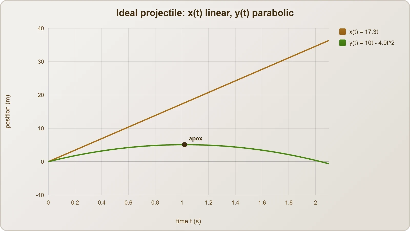
This independence means a projectile's horizontal position-time graph is a straight line when air resistance is ignored, while its vertical graph is a parabola. Reading them side by side, a learner immediately sees that horizontal velocity stays constant while vertical velocity changes steadily. The visual contrast reinforces the underlying physics far more effectively than equations alone.

From Vectors to Curves

Every vector quantity in a plane can be decomposed into scalar components, and each component can be plotted against time. The resulting family of graphs forms a complete graphical portrait of the motion. Position components, velocity components, and acceleration components each contribute a distinct layer of information to that portrait.

When these layers are stacked, a rich diagnostic picture emerges. A curved position graph signals changing velocity; a linear velocity graph signals constant acceleration; a horizontal acceleration graph signals zero acceleration in that direction. Learning to read these signatures is the central skill of this lesson and the bridge to more advanced kinematics.

Position-Time Graphs for Each Component

The position-time graph is the most intuitive entry point into graphical analysis because it resembles a map of where the object has been. For motion in a plane, two such graphs are drawn side by side, one for the horizontal coordinate and one for the vertical coordinate. Together they trace the object's itinerary through space.

Reading the Horizontal Position Graph

For a projectile launched with no air resistance, the horizontal position graph is a straight line whose slope equals the constant horizontal velocity ##v_x##. The equation governing this line is simply ##x = x_0 + v_x t##, a linear relationship that beginners can verify by inspection. A steeper line means a faster horizontal motion.

Interpreting the intercept is equally important. The value of ##x## at ##t = 0## gives the initial horizontal position, which may be zero or any chosen reference point. If the line slopes downward, the object moves in the negative x-direction, and the slope carries a negative sign that encodes direction as well as speed.

Reading the Vertical Position Graph

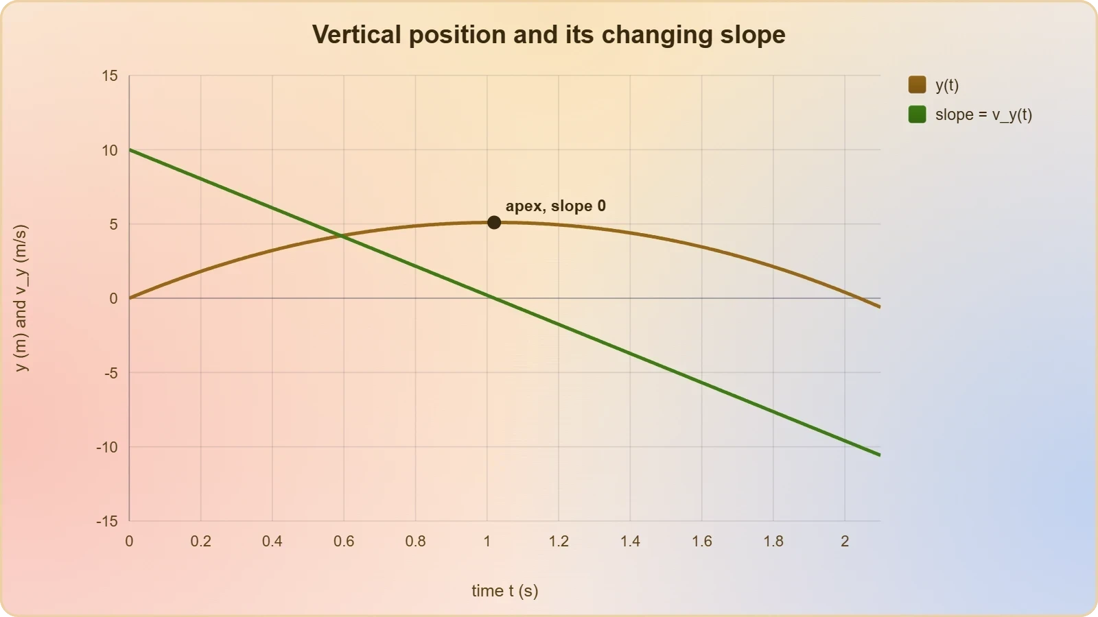
The vertical position graph for a projectile is a downward-opening parabola, reflecting the constant downward acceleration due to gravity. Its equation takes the familiar form ##y = y_0 + v_{y0} t - \tfrac{1}{2} g t^2##, where the quadratic term bends the curve progressively. The vertex marks the highest point of the trajectory.

Slope analysis on this curve is revealing. Near the launch, the slope is positive and steep, indicating upward motion; at the apex, the slope momentarily vanishes; afterward, the slope turns negative as the object descends. The changing slope is a direct visual representation of changing vertical velocity.

Velocity-Time Graphs and Their Slopes

Velocity-time graphs carry the analysis one derivative deeper, converting position information into rates of change. For each component, the velocity graph's slope yields the corresponding acceleration component, while the area beneath the curve yields displacement. These two operations, slope and area, form the twin pillars of graphical kinematics.

Horizontal Velocity Graph

In ideal projectile motion, the horizontal velocity graph is a horizontal line at the value ##v_x##, because no horizontal force acts once the object is airborne. Its slope is zero, confirming zero horizontal acceleration. The area under this line over a time interval equals the horizontal displacement during that interval.

Real-world complications such as air resistance bend this line slightly downward, producing a small negative slope that represents deceleration. Recognising this deviation from the ideal case is valuable, because it teaches learners to distinguish textbook models from physical reality. The graph becomes a diagnostic tool for identifying drag effects.

Vertical Velocity Graph

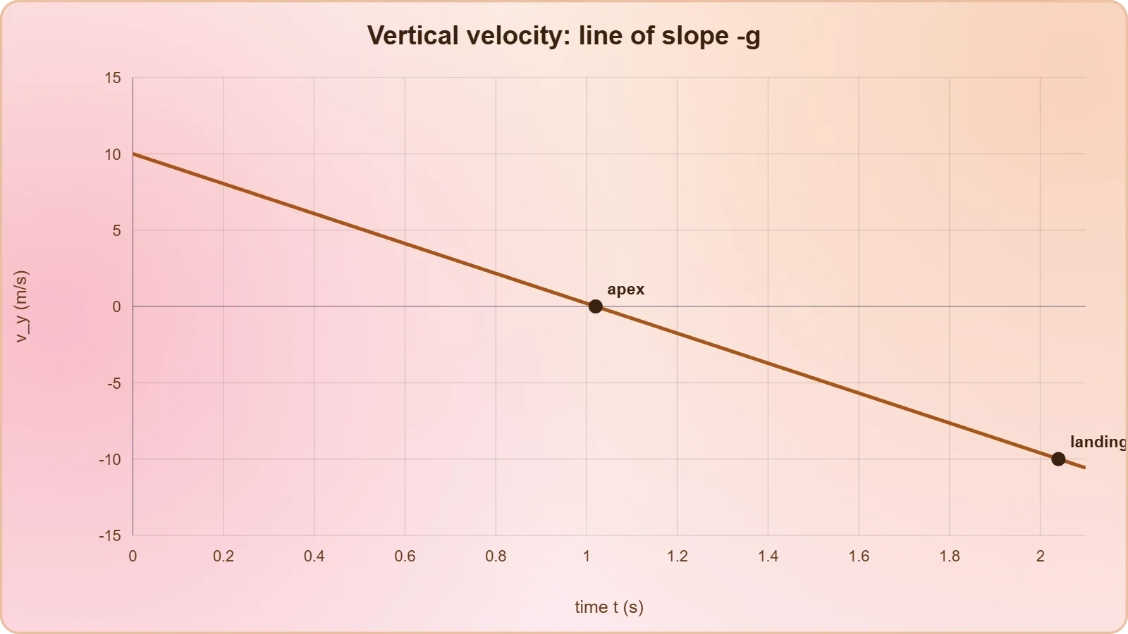
The vertical velocity graph is a straight line with slope ##-g##, descending steadily from its initial positive value through zero at the apex and into negative territory during descent. This single line elegantly captures the entire vertical history of a projectile. Its slope is constant, confirming uniform vertical acceleration.

Area calculations on this graph are especially instructive. The area between the line and the time axis, taken with proper signs, gives the vertical displacement. Positive and negative areas above and below the axis cancel appropriately, so the net area from launch to landing returns to zero for a projectile landing at its starting height.

Acceleration Graphs and the Second Derivative

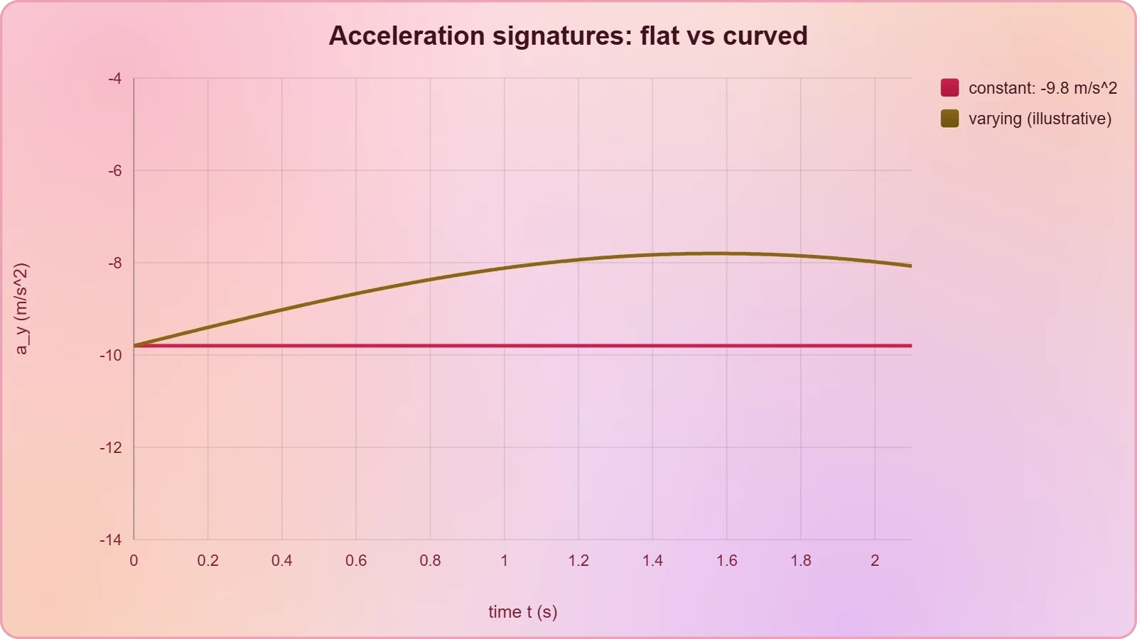
Acceleration-time graphs complete the graphical hierarchy, representing the second derivative of position with respect to time. For projectile motion, the horizontal acceleration graph is a flat line at zero, while the vertical acceleration graph is a flat line at ##-g##. Their simplicity belies their explanatory power.

Constant Acceleration Signatures

A horizontal line on an acceleration-time graph indicates constant acceleration, and its height gives the magnitude and sign of that acceleration. In projectile motion, the vertical acceleration graph sits at approximately ##-9.8 \text{ m/s}^2## throughout the flight. This constancy is the graphical fingerprint of uniform acceleration.

When acceleration is not constant, the graph becomes a curve, and the analysis grows richer. A changing acceleration graph signals that forces are varying with time, as happens with air resistance or rocket thrust. Recognising these signatures prepares learners for dynamics topics where forces themselves become the focus.

Connecting the Three Graph Families

The three graph families form an integrated system in which each level is the slope of the level above it. Position slopes to velocity, velocity slopes to acceleration, and acceleration slopes to jerk. Conversely, each level is the area under the level below it, creating a bidirectional web of graphical relationships.

Mastering this web allows a learner to move fluidly between representations. Given any one graph, the others can be reconstructed through slope and area operations, provided initial conditions are known. This fluency is precisely what the next lesson will exploit when vectors are applied to real-world navigation and engineering problems.

Worked Example: Decoding a Projectile's Graphs

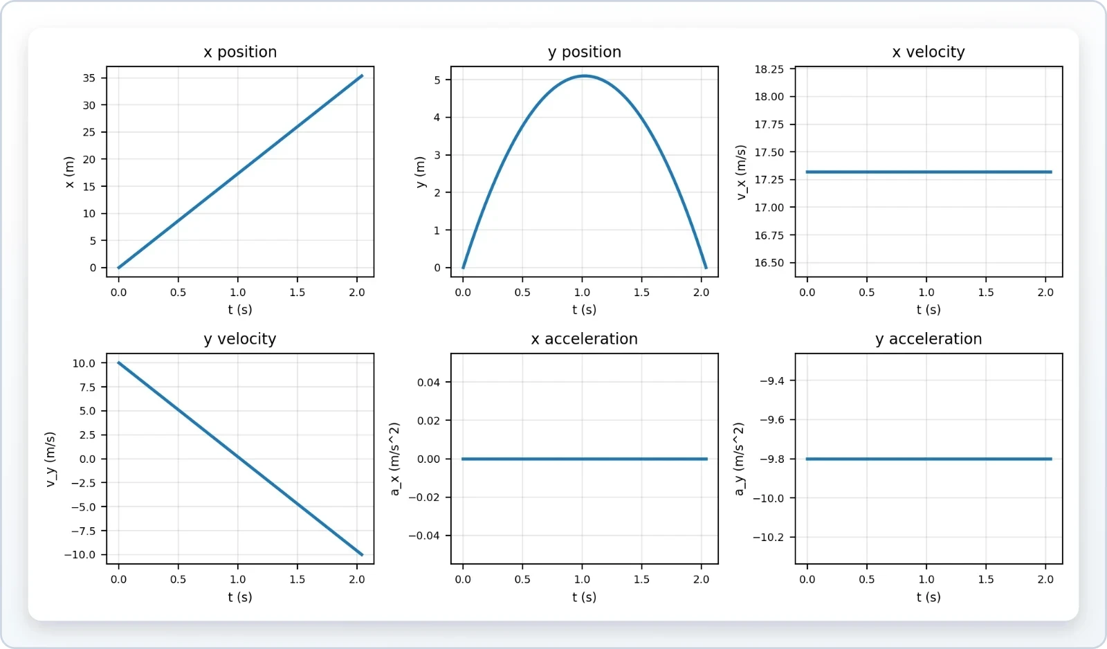
A concrete example consolidates the abstract principles. Consider a ball launched at ##20 \text{ m/s}## at an angle of ##30^\circ## above the horizontal from ground level, with air resistance ignored. Its initial velocity components are ##v_x = 20\cos 30^\circ \approx 17.3 \text{ m/s}## and ##v_{y0} = 20\sin 30^\circ = 10 \text{ m/s}##.

Constructing the Graphs

The horizontal position graph is a straight line rising at ##17.3 \text{ m/s}##, while the vertical position graph is a parabola peaking at ##t = v_{y0}/g \approx 1.02 \text{ s}##. The vertical velocity graph descends from ##+10## to ##-10 \text{ m/s}## over roughly ##2.04 \text{ s}##. Each graph can be sketched from these anchor values.

Acceleration graphs are trivially flat: zero horizontally and ##-9.8 \text{ m/s}^2## vertically. The complete set of six graphs, two per quantity, forms a coherent portrait. Learners should practise sketching all six from a single set of initial conditions until the process becomes automatic.

Extracting Numerical Answers

Graphical analysis yields numerical answers through slope and area. The area under the vertical velocity graph from launch to apex gives the maximum height, approximately ##5.1 \text{ m}##. The total area from launch to landing, accounting for sign, returns to zero, confirming the symmetric flight.

The horizontal displacement follows from the area under the horizontal velocity graph over the total flight time of about ##2.04 \text{ s}##, giving a range near ##35.3 \text{ m}##. These results match the standard kinematic equations, validating the graphical method. The graphs and equations are two languages describing the same physics.

Common Pitfalls and How to Avoid Them

Graphical analysis rewards precision and punishes carelessness, and several recurring errors trip up learners. The most frequent is confusing the slope of a position-time graph with position itself, or reading a velocity value directly from a position axis. Careful axis labelling prevents most of these mistakes.

Sign Errors and Axis Confusion

Signs carry directional information in two-dimensional motion, and ignoring them corrupts every subsequent calculation. A negative slope on a position graph means motion in the negative direction, not a smaller speed. Similarly, areas below the time axis represent negative displacement and must be subtracted, not added.

Axis confusion arises when learners forget which component a graph represents. Labelling each graph clearly, for example "x-position versus time," eliminates ambiguity. Consistent conventions, such as taking rightward and upward as positive, keep the analysis coherent across all six graphs.

Misreading Curvature and Tangents

Curvature on a position-time graph is often misread as a change in direction, when it actually indicates changing speed. A parabola opening upward means acceleration is positive, not that the object has reversed course. Distinguishing curvature from turning points requires attention to the slope's sign and magnitude separately.

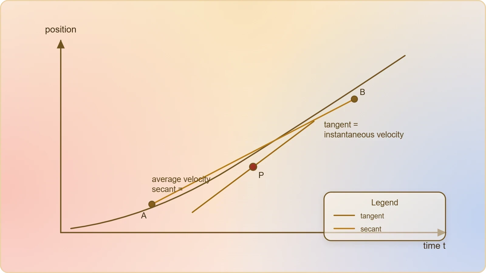
Tangent lines provide instantaneous velocity, while secant lines provide average velocity over an interval. Confusing the two leads to incorrect answers when the motion is accelerated. Drawing tangents carefully at several points builds intuition for how instantaneous velocity evolves along a curved path.

Preparing for Real-World Vector Applications

Graphical analysis is more than an academic exercise; it is the visual grammar that real-world vector problems are written in. Navigation charts, sports trajectory analyses, and engineering design plots all rely on the same slope-and-area reasoning developed here. The next lesson extends these skills to contexts where vectors describe actual journeys and forces.

From Graphs to Practical Reasoning

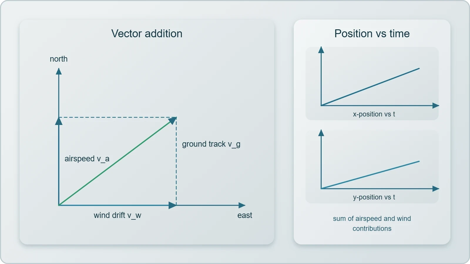
Consider a drone navigating a crosswind. Its ground-track position graph is the vector sum of its airspeed motion and the wind's drift, and component graphs reveal each contribution separately. Reading such graphs lets an operator predict arrival points and correct course before errors accumulate.

Sports analytics offers another vivid application. A basketball's shot can be tracked with high-speed cameras, producing position and velocity graphs for both components. Coaches use the vertical velocity graph to assess release angle and the horizontal graph to evaluate consistency, translating graphical features directly into performance feedback.

Building Toward the Next Lesson

The skills practised here, decomposing motion into components and reading their graphs, are precisely the tools needed when vectors enter real-world contexts. Whether the problem involves river crossings, aircraft headings, or robotic path planning, the graphical intuition developed in this lesson provides a reliable foundation for interpretation.

As you move forward, keep sketching graphs alongside your equations. The habit of visualising each component separately will make complex vector problems tractable and reveal physical insights that algebra alone might hide. Graphical analysis is not a detour from vector reasoning; it is the clearest expression of it.