Motion in a Plane: Advanced Problem Set

Advanced problem sets in two-dimensional kinematics are where the separate threads of a course finally weave together. Students who have mastered vector decomposition, projectile trajectories, and centripetal acceleration in isolation often discover that real examination questions demand all three at once, sometimes within a single scenario. This lesson deliberately assembles that kind of intellectual pressure, presenting problems that refuse to sit neatly inside one chapter heading.

The pedagogical logic here is cumulative rather than additive. Each problem is constructed so that a careless assumption about one sub-concept corrupts the entire solution, forcing learners to audit their reasoning at every stage. A projectile launched from a moving platform, for instance, requires relative velocity reasoning before the familiar range equation can even be applied. Such layered demands mirror how physics is actually practised, where clean textbook conditions rarely survive contact with a real apparatus.

What follows is a structured walkthrough of the problem-solving architecture that separates competent students from exceptional ones. We examine vector superposition under constraint, projectile motion with non-trivial launch conditions, circular motion coupled to tangential dynamics, and the error analysis that keeps numerical answers honest. Each section pairs worked reasoning with the diagnostic habits that prevent silent mistakes from propagating through a solution.

Building a Problem-Solving Architecture for Two-Dimensional Motion

Before touching a single equation, the advanced solver performs a structural read of the problem. This means identifying which quantities are given, which are implied by geometry, and which are genuinely unknown rather than merely unlabelled. Beginners rush to formulas; experienced problem solvers first map the physical situation onto a coordinate system that minimises algebraic pain.

Choosing Coordinates That Simplify the Algebra

Coordinate selection is not cosmetic. Tilting axes to align with an inclined plane, for example, converts a two-component acceleration problem into a single-component one, eliminating an entire class of sign errors. The same principle applies to circular motion problems where radial and tangential directions deserve their own basis vectors rather than Cartesian defaults.

A useful discipline is to sketch the free-body diagram and the kinematic vectors on the same page before writing anything symbolic. When the acceleration vector and the chosen axis disagree in direction, the sign convention becomes visible immediately. Students who skip this step frequently produce answers that are numerically plausible but physically inverted.

Decomposing Compound Motion into Independent Components

The independence of horizontal and vertical motion remains the workhorse principle of projectile analysis, yet advanced problems stress it in unfamiliar ways. A ball thrown from a cliff toward a moving target couples constant-velocity horizontal motion with uniformly accelerated vertical motion, and the time of flight is governed entirely by the vertical equation.

Formally, the position vector evolves as a superposition of two independent one-dimensional motions. The horizontal component obeys ##x(t) = x_0 + v_{0x} t## while the vertical follows ##y(t) = y_0 + v_{0y} t - \tfrac{1}{2} g t^2##. Neither equation knows about the other, which is precisely why the decomposition works so reliably across problem types.

Vector Superposition Under Real Constraints

Textbook vector addition usually involves tidy triangles with pleasant angles. Advanced problems replace these with river crossings, wind corrections, and aircraft headings where the resultant direction is prescribed rather than the component magnitudes. The solver must invert the usual logic, working backward from a required resultant to find the input vector.

River Crossing and Relative Velocity Problems

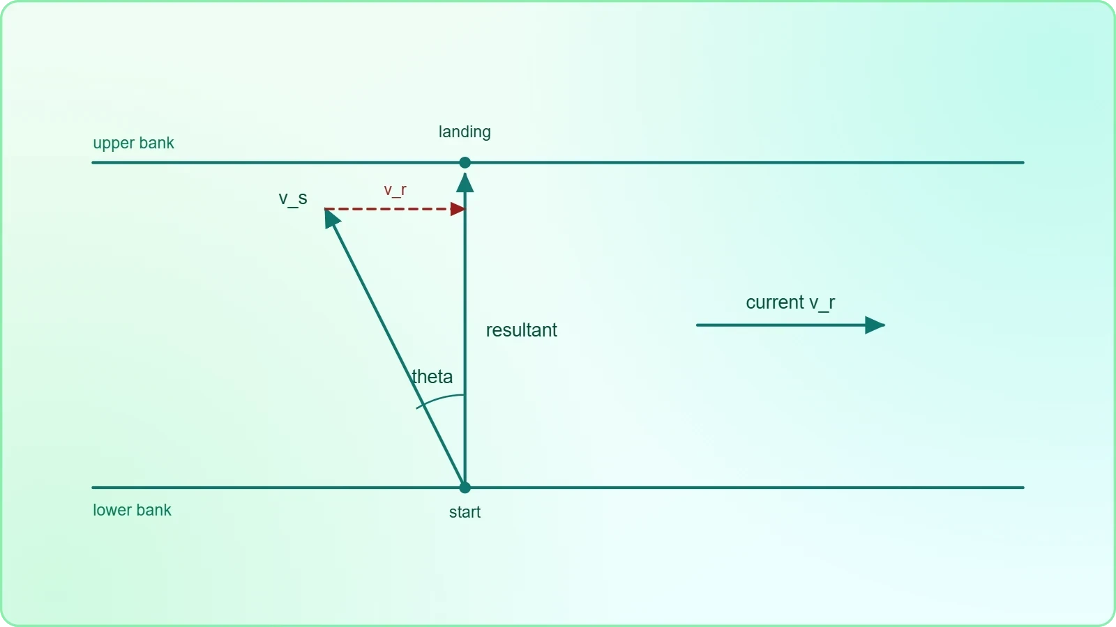
A swimmer aiming straight across a flowing river never lands directly opposite the start. The current drags the path downstream, and the crossing time depends only on the swimmer's speed perpendicular to the bank. This asymmetry between time and displacement is the conceptual heart of every relative velocity problem.

To land at a specific point, the swimmer must angle upstream by an amount satisfying ##\sin\theta = v_r / v_s##, where ##v_r## is the river speed and ##v_s## the swimmer's speed in still water. If ##v_r \geq v_s##, no heading achieves a perpendicular crossing, and the problem becomes one of minimising drift rather than eliminating it.

Resolving Forces and Velocities Simultaneously

Some problems present a body subject to both kinematic and dynamic constraints, such as a block sliding on an accelerating wedge. Here the velocity decomposition and the force decomposition must share the same coordinate basis, or the resulting equations become inconsistent. Consistency of basis is the silent requirement behind every correct multi-constraint solution.

Writing the constraint equation explicitly, such as ##a_{block} = a_{wedge} + a_{rel}##, forces the solver to declare which frame each acceleration belongs to. This declaration prevents the classic error of mixing laboratory-frame and wedge-frame quantities inside a single Newton's second law statement.

Projectile Problems with Non-Standard Launch Conditions

Standard projectile problems launch from ground level onto flat terrain. Advanced variants launch from height, target elevated positions, or involve moving platforms, and each variation shifts which equation should be solved first. Recognising the correct entry point into the mathematics is the skill being tested.

Launch from Height and Elevated Targets

When a projectile is fired from a cliff toward a target below, the vertical displacement is negative and the quadratic in time may yield one positive and one negative root. Only the positive root is physical, and discarding the other is not a formality but a statement about causality. Students who retain both roots occasionally report absurd negative flight times.

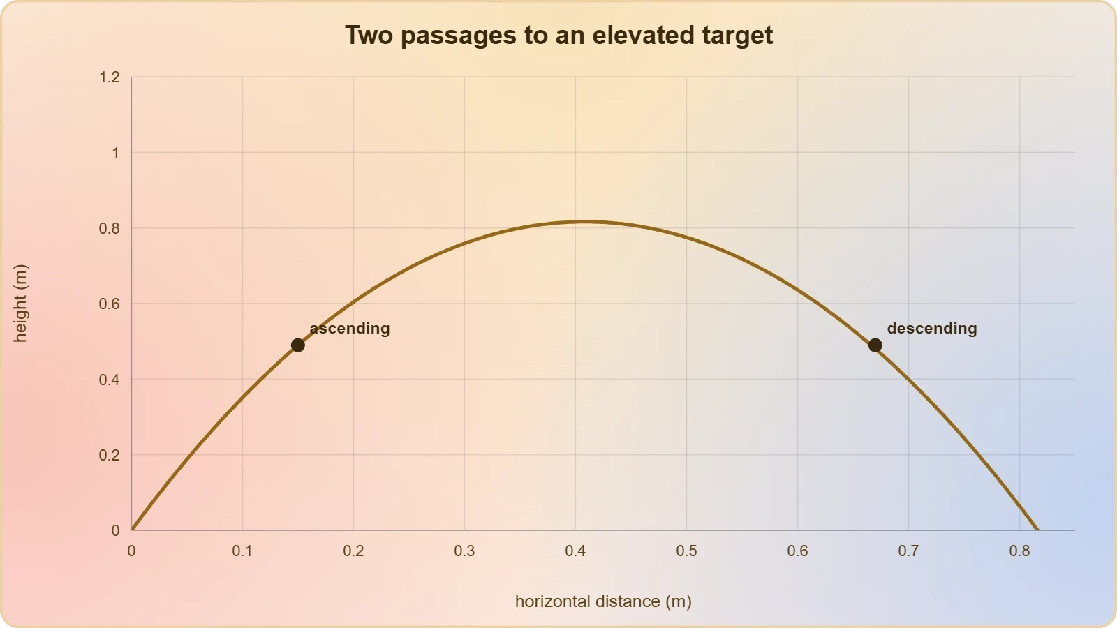
For elevated targets, the projectile may reach the target height twice, once ascending and once descending. The problem statement must specify which passage is intended, and the range equation alone cannot distinguish them. This ambiguity is a favourite device in competitive examinations because it rewards careful reading over formula recall.

Trajectory Equations and Envelope Analysis

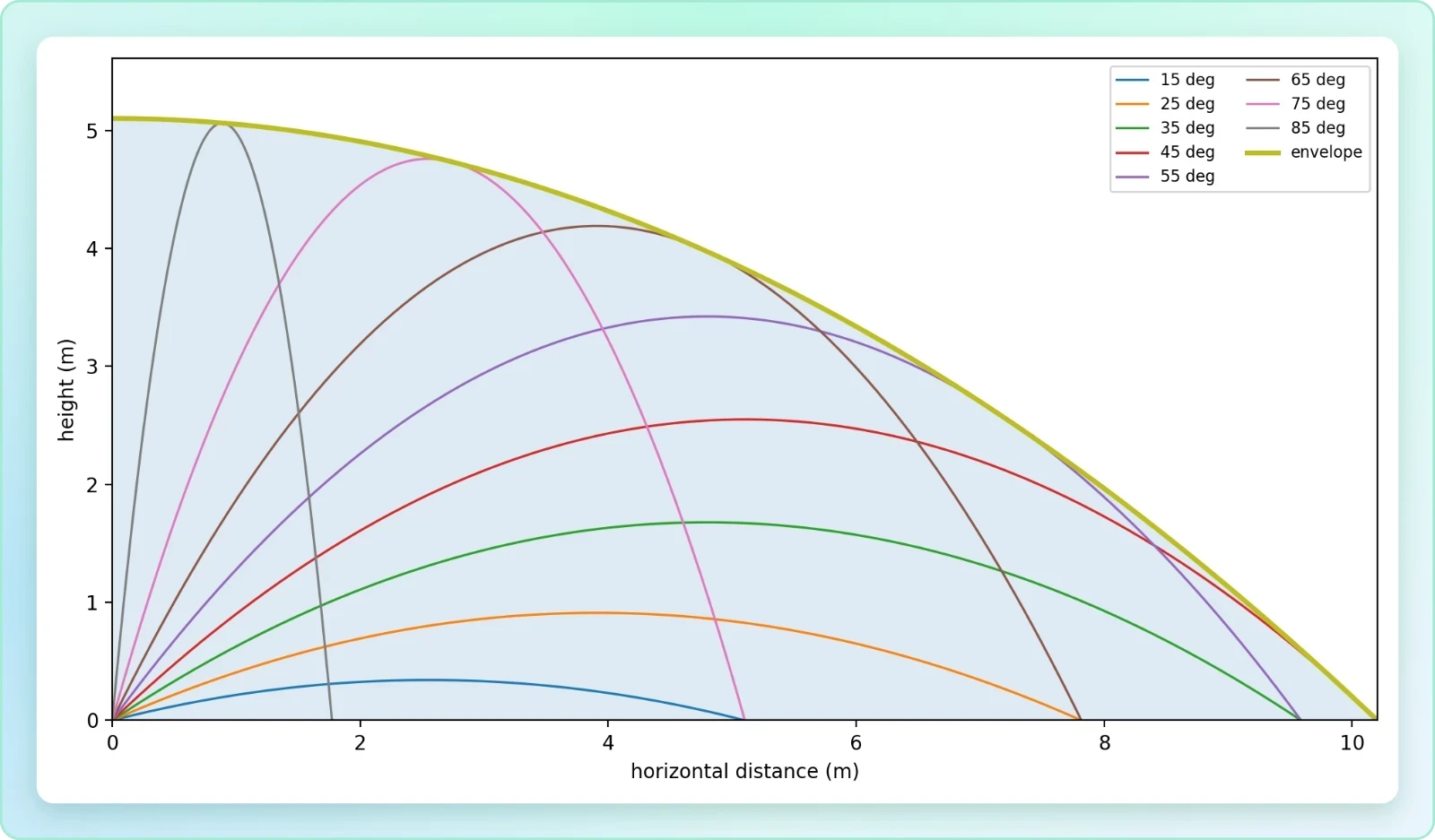
Eliminating time from the parametric equations yields the trajectory parabola, a compact description of the entire path. The equation takes the form of a downward-opening parabola whose coefficients encode launch speed and angle. From this single expression, questions about maximum height, range, and impact angle can all be answered by differentiation.

The envelope of all possible trajectories at fixed speed defines the boundary of reachable space, known as the parabola of safety. Any target inside this boundary can be hit with two complementary launch angles, while targets outside it are unreachable regardless of aim. This geometric insight converts a family of problems into a single inequality test.

Circular Motion Coupled with Tangential Dynamics

Uniform circular motion is comfortable territory, but advanced problems introduce tangential acceleration, variable speed, and friction that must supply the centripetal force. A car on a banked curve at the verge of slipping, or a bead sliding on a rotating hoop, demands simultaneous radial and tangential force analysis. The two directions are orthogonal, yet their equations are coupled through the speed.

Banked Curves, Friction Limits, and Design Speed

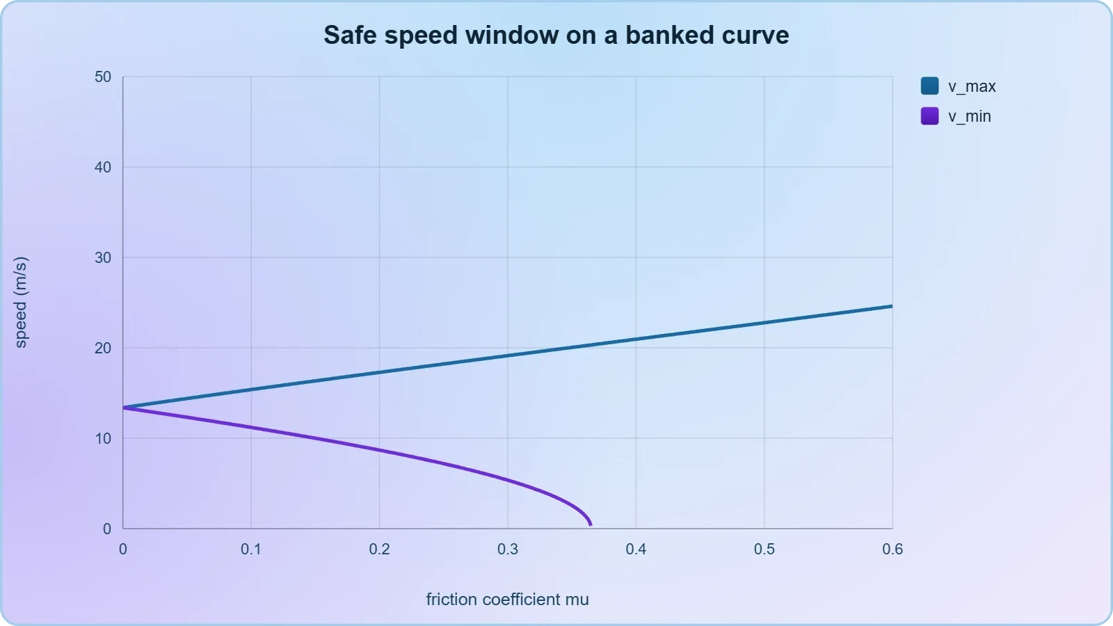
On a frictionless banked curve, the design speed satisfies ##\tan\theta = v^2/(rg)##, the angle at which the normal force alone provides the required centripetal component. Real roads add friction, widening the safe speed window in both directions. The maximum safe speed combines both contributions, while the minimum speed subtracts them.

Solving the coupled equations requires resolving the normal force and friction into radial and vertical components, then eliminating the normal force between them. The resulting expression for maximum speed is ##v_{max} = \sqrt{rg(\tan\theta + \mu)/(1 - \mu\tan\theta)}##, which reduces gracefully to the frictionless case when ##\mu = 0##.

Non-Uniform Circular Motion and Angular Acceleration

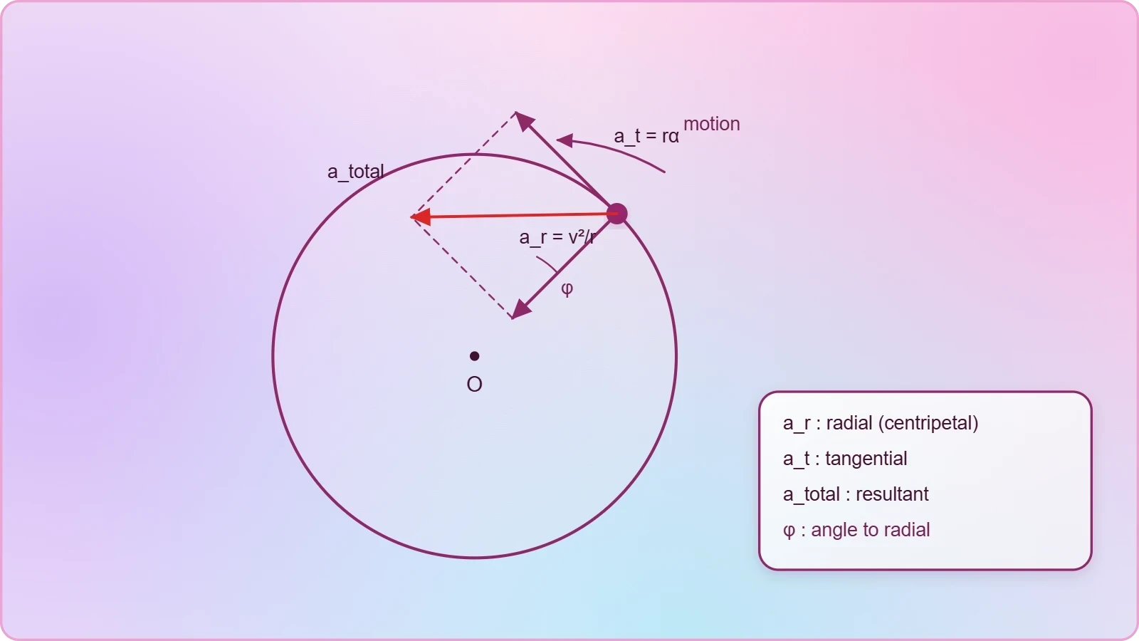
When speed changes along the circle, a tangential acceleration ##a_t = r\alpha## appears alongside the radial term ##a_r = v^2/r##. The total acceleration is their vector sum, and its direction no longer points toward the centre. Problems asking for the angle between total acceleration and the radius test precisely this composition.

The angular kinematics mirror linear kinematics, with ##\omega = \omega_0 + \alpha t## and ##\theta = \omega_0 t + \tfrac{1}{2}\alpha t^2##. Recognising this correspondence lets students transfer familiar techniques directly, provided they remember that the centripetal term depends on the instantaneous angular speed rather than any average.

Integrating Concepts: Multi-Stage Motion Problems

The most demanding problems chain several regimes together, such as a projectile that lands on a rotating platform or a bead that leaves a circular track and becomes a projectile. These composite scenarios require the solver to identify transition points where one set of equations hands over to another. The handover conditions, usually position and velocity continuity, are where marks are won or lost.

Transition Between Constrained and Free Motion

When a bead loses contact with a circular hoop, the normal force vanishes at the transition instant. That condition, ##N = 0##, determines the speed and angle at which free flight begins. From that point, the bead obeys projectile equations with initial conditions inherited from the circular phase.

Setting up such problems requires computing the launch velocity vector from the circular motion, then feeding it into the projectile equations. The angle of the velocity at release is tangential to the circle, which is perpendicular to the radius. Missing this geometric fact sends the entire subsequent calculation astray.

Worked Composite Example with Verification

Consider a ball rolling off a frictionless quarter-pipe of radius ##R## and landing on the ground below. Energy conservation gives the launch speed ##v = \sqrt{2gR}##, and the launch angle is horizontal. The projectile phase then follows standard equations with zero initial vertical velocity.

import math

g = 9.81
R = 2.0
h = 3.0  # height of pipe exit above ground

v_launch = math.sqrt(2 * g * R)
t_fall = math.sqrt(2 * h / g)
x_range = v_launch * t_fall

print(f"Launch speed: {v_launch:.2f} m/s")
print(f"Flight time:  {t_fall:.2f} s")
print(f"Range:        {x_range:.2f} m")

Verification follows by checking limiting cases: if ##h## approaches zero, the range should vanish, and if ##R## grows, the range should scale as its square root. Such sanity checks catch unit errors and algebraic slips that survive dimensional analysis. A solution that fails a limiting case is wrong, however elegant its derivation.

Error Analysis and Numerical Sanity Checks

Advanced problems often carry measured data, and the final answer must reflect the precision of its inputs. Reporting a range of 47.382 metres from a launch speed quoted to two significant figures is a category error, not merely a stylistic one. Significant figures and uncertainty propagation belong in every serious solution.

Significant Figures and Uncertainty Propagation

When quantities are multiplied or divided, their relative uncertainties add in quadrature, giving ##\dfrac{\delta z}{z} = \sqrt{(\dfrac{\delta x}{x})^2 + (\dfrac{\delta y}{y})^2}## for ##z = xy##. For sums and differences, absolute uncertainties combine instead. Choosing the wrong rule is among the most common errors in laboratory-style kinematics questions.

Angles introduce a subtlety because trigonometric functions amplify or suppress uncertainty depending on the operating point. Near 45 degrees, the sine changes slowly, so angular uncertainty barely affects range; near zero or ninety degrees, the sensitivity is far higher. Recognising this asymmetry guides sensible experimental design.

Limiting Cases as a Verification Tool

Every derived formula should be interrogated at its boundaries. Setting the launch angle to zero should recover horizontal projection, setting gravity to zero should produce straight-line motion, and setting friction to infinity should freeze the system. A formula that misbehaves at these limits contains an error somewhere in its derivation.

Dimensional analysis provides a complementary check that costs almost nothing. If the units of a candidate expression do not reduce to metres per second squared for an acceleration, the algebra is wrong regardless of how plausible the number looks. Combining dimensional checks with limiting cases catches the overwhelming majority of silent mistakes.

Preparing for the Course Summary

This problem set deliberately gathers the course's central techniques into single scenarios, and that integration is itself the lesson. Students who can move fluidly between vector decomposition, projectile analysis, and circular dynamics have internalised the subject rather than memorised its chapters. The next lesson consolidates these threads into a coherent summary and points toward further study.

Consolidating Techniques Across the Course

A useful revision strategy is to catalogue every problem type encountered and note which principles each one activates. The catalogue reveals that a small set of ideas, chiefly independence of components and continuity at transitions, underlies nearly every question. Recognising this economy of concepts reduces the apparent volume of material dramatically.

Students should also revisit their earlier mistakes, since misconceptions corrected in the previous lesson tend to resurface under examination pressure. Deliberately re-solving a problem that once defeated you is a more efficient use of time than attempting many fresh problems of the same type. Depth beats breadth in the final stages of preparation.

Looking Ahead to Future Directions

Beyond this course lie rotating reference frames, Coriolis effects, and the full machinery of Newtonian mechanics in three dimensions. Each builds directly on the two-dimensional foundations rehearsed here, so fluency with these problem sets pays dividends later. The summary lesson will map that trajectory and suggest where to direct further effort.