Motion in a Plane: Mathematical Foundations

Motion in a plane rests on a compact mathematical toolkit that students often meet piecemeal: sines and cosines in trigonometry class, arrows and components in a physics lecture, and coordinate geometry somewhere in between. Lesson 27 of this thirty-part course gathers those threads into a single, coherent framework. The aim is not to introduce new physical phenomena but to sharpen the instruments used to describe them, so that projectile paths and circular trajectories become calculations rather than guesswork.

Because the preceding lesson examined laboratory and real-world experiments, the emphasis here shifts deliberately toward abstraction. Measurements taken in the field only become predictive when they are expressed through angles, magnitudes, and components. This lesson therefore revisits the mathematics that converts raw observation into a solvable model, and it does so with the beginner firmly in mind. Every definition is paired with a worked illustration drawn from two-dimensional motion.

The material also prepares the ground for the next lesson on common misconceptions. Many persistent errors in plane kinematics, from sign confusion to the false belief that a projectile's horizontal velocity decays, trace back to shaky mathematical habits. By consolidating trigonometry and vector algebra now, learners arrive at that diagnostic discussion equipped to recognise exactly where their reasoning slipped. The treatment below is self-contained, sequential, and built for steady, confident progress.

Why Plane Motion Demands a Mathematical Language

Two-dimensional motion cannot be captured by a single number, because position, velocity, and acceleration each possess both size and direction. Mathematics supplies the vocabulary for that duality. Trigonometry resolves a slanted quantity into perpendicular parts, while vector algebra governs how those parts combine, subtract, and scale. Together they transform a physical situation into equations that can be solved systematically.

Scalars, Vectors, and the Meaning of Direction

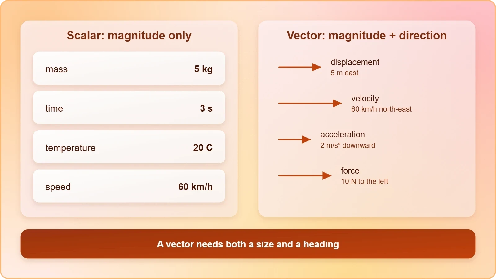
A scalar is fully specified by magnitude alone: mass, time, temperature, and speed all qualify. A vector requires direction as well, so displacement, velocity, acceleration, and force belong to this second class. Writing a vector as ##\vec{A}## signals that the arrow carries orientation, not merely length. Confusing the two categories is the first mathematical trap in plane motion.

Speed and velocity illustrate the distinction concretely. A car travelling at sixty kilometres per hour has a speed; the same car heading north-east at sixty kilometres per hour has a velocity. The magnitude of velocity is speed, but the reverse inference fails because direction is discarded. Every vector equation in this course preserves that directional information until the final numerical step.

Coordinate Frames and the Choice of Axes

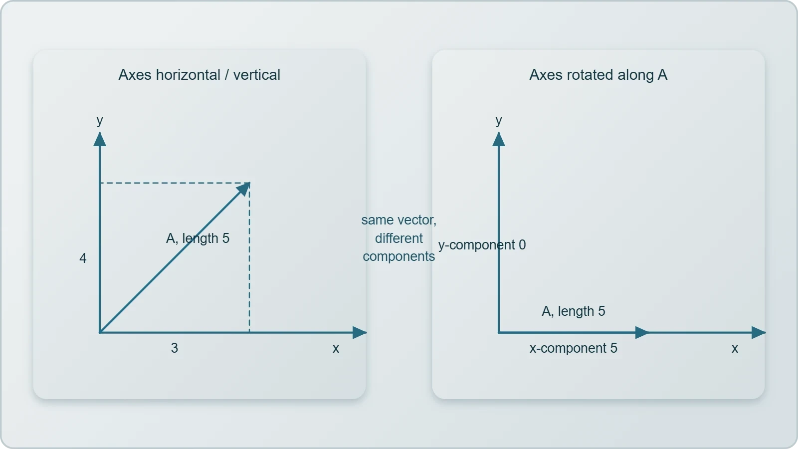
Vectors exist independently of any coordinate system, yet calculations demand one. Choosing axes is therefore a strategic decision rather than a formality. Aligning the x-axis with the direction of initial motion often eliminates unnecessary terms, while tilting axes to match an inclined surface can simplify otherwise awkward components. Skilled problem-solvers select frames that minimise algebra.

Once axes are fixed, a vector acquires components that depend on the chosen orientation. The same displacement may read as ##(3, 4)## in one frame and ##(5, 0)## in another rotated by the appropriate angle. Physical conclusions remain invariant under such rotations, which is precisely why the freedom to choose axes is legitimate. The underlying reality does not change when the description does.

Trigonometry as the Bridge to Components

Right-triangle trigonometry converts between a vector's slanted description and its perpendicular parts. The sine, cosine, and tangent ratios connect an angle to side lengths, and in physics those sides become components. Mastery here removes most of the friction from projectile and circular-motion problems, because nearly every such problem begins by resolving a vector into horizontal and vertical pieces.

Sine, Cosine, and Tangent in Physical Context

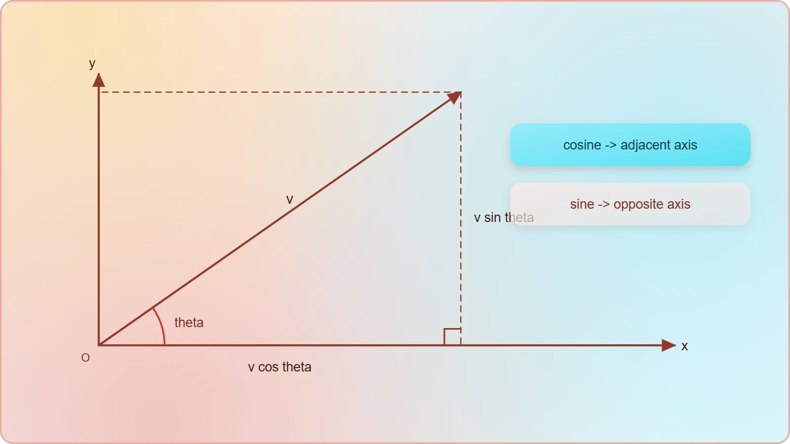
For a right triangle with angle ##\theta##, the ratios are defined as ##\sin\theta = \dfrac{\text{opposite}}{\text{hypotenuse}}##, ##\cos\theta = \dfrac{\text{adjacent}}{\text{hypotenuse}}##, and ##\tan\theta = \dfrac{\text{opposite}}{\text{adjacent}}##. These are dimensionless numbers, which is why they can multiply a velocity or a force without altering its units. The angle itself carries no units in the ratio.

A velocity of magnitude ##v## inclined at angle ##\theta## above the horizontal resolves into ##v_x = v\cos\theta## and ##v_y = v\sin\theta##. The cosine attaches to the axis adjacent to the angle, the sine to the axis opposite it. Learners who memorise this pairing as a rule rather than a derivation frequently swap the two under exam pressure, so deriving it once from a sketch is worthwhile.

Standard Angles and the Unit Circle

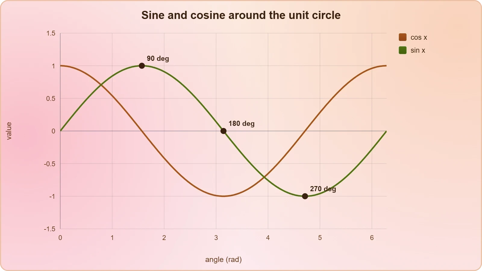
Certain angles recur so often that their trigonometric values deserve instant recall. At thirty degrees, sine is one-half and cosine is ##\dfrac{\sqrt{3}}{2}##; at forty-five degrees both equal ##\dfrac{\sqrt{2}}{2}##; at sixty degrees the values exchange. These exact forms keep intermediate work clean and reveal when a result simplifies unexpectedly.

The unit circle extends the definitions beyond acute angles, assigning signs according to quadrant. A velocity pointing into the second quadrant has a negative horizontal component and a positive vertical one, a fact the circle makes visually obvious. Recognising these sign patterns early prevents the algebraic contradictions that plague careless component work later in the course.

Vector Algebra: Addition, Subtraction, and Resolution

Vectors obey their own arithmetic, and that arithmetic differs from ordinary number work in one crucial respect: direction participates in every operation. Adding two vectors is not simply adding their magnitudes, because opposing arrows partially cancel. The two standard methods, graphical and component-wise, produce identical results, and fluency with both builds genuine intuition about plane motion.

The Triangle and Parallelogram Methods

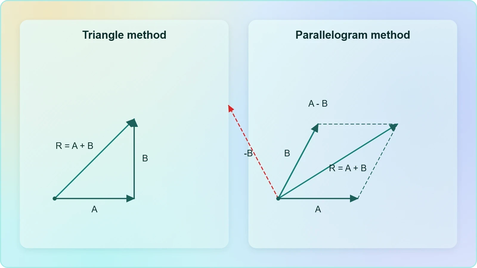
Placing the tail of one vector at the tip of another and drawing the resultant from first tail to final tip gives the triangle method. The parallelogram method instead places both tails together and completes the figure, with the diagonal representing the sum. Both are visual, approximate, and excellent for checking whether a computed answer is plausible.

Subtraction follows by reversing the vector being removed before adding. The difference ##\vec{A} - \vec{B}## equals ##\vec{A} + (-\vec{B})##, where ##-\vec{B}## has identical magnitude but opposite direction. This operation underlies relative velocity problems, where the velocity of one body as seen from another is the vector difference of their velocities.

Component Addition and the Resultant Magnitude

Component addition is the workhorse method because it reduces vector sums to ordinary arithmetic. Each vector is resolved into x and y parts, the parts are summed separately, and the resultant is reconstructed. For vectors ##\vec{A}## and ##\vec{B}##, the resultant components are ##R_x = A_x + B_x## and ##R_y = A_y + B_y##.

The magnitude and direction of the resultant then follow from the Pythagorean theorem and the inverse tangent:

The inverse tangent requires care, since calculators return values only between ##-90°## and ##90°##. When ##R_x## is negative, the true angle lies in the second or third quadrant and must be adjusted by adding or subtracting ##180°##. This single adjustment resolves a large share of sign errors in student work.

Applying the Toolkit to Projectile and Circular Problems

Mathematics earns its place when it shortens a physical solution. Projectile motion separates into independent horizontal and vertical descriptions, each governed by simple equations once components are known. Uniform circular motion instead demands an understanding of how a changing direction produces acceleration even at constant speed. Both cases reward the trigonometric and vector habits built above.

Resolving Initial Velocity in Projectile Motion

A projectile launched at speed ##u## and angle ##\theta## begins with ##u_x = u\cos\theta## and ##u_y = u\sin\theta##. The horizontal component persists unchanged, while the vertical component evolves under gravity. This decomposition converts a curved path into two straight-line problems solved with familiar one-dimensional equations.

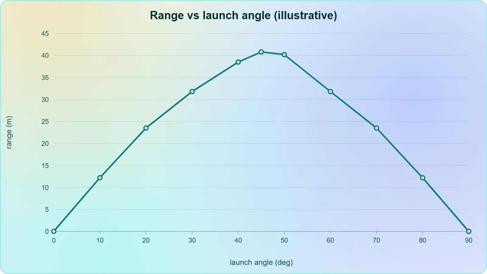
The time of flight follows from the vertical motion alone, since the projectile returns to its launch height when the vertical displacement vanishes. Setting ##u_y t - \dfrac{1}{2}gt^2 = 0## yields ##t = \dfrac{2u\sin\theta}{g}##. The horizontal range then becomes ##R = \dfrac{u^2 \sin 2\theta}{g}##, a result whose symmetry about forty-five degrees is a direct consequence of trigonometry.

Angles, Radians, and Circular Kinematics

Circular motion introduces angular quantities, and these require radian measure rather than degrees. One radian subtends an arc equal to the radius, so a full revolution equals ##2\pi## radians. Angular velocity ##\omega## relates to linear speed through ##v = \omega r##, a relation that only holds cleanly when the angle is expressed in radians.

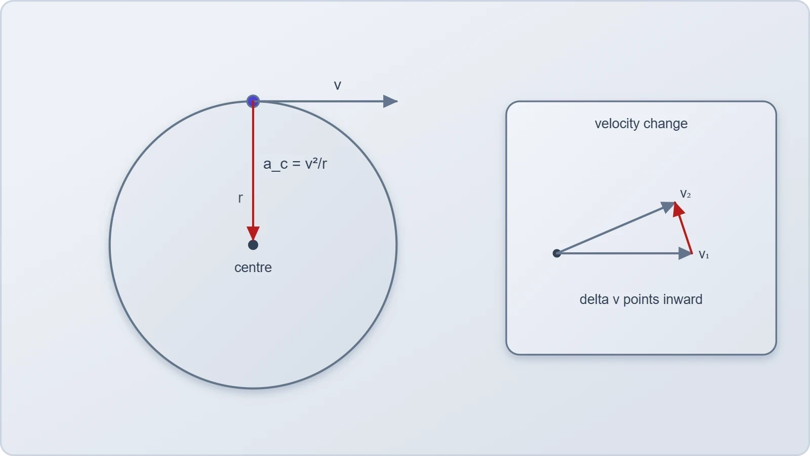
Centripetal acceleration points toward the centre with magnitude ##a_c = \dfrac{v^2}{r} = \omega^2 r##. The direction changes continuously, which is why acceleration exists despite constant speed. Vector language captures this elegantly: the velocity vector rotates, and its rate of change is perpendicular to itself, pointing inward along the radius.

Computational Practice: Turning Formulas into Code

Modern learners benefit from translating these formulas into executable code, because a program exposes every hidden assumption. Writing a short script to resolve a vector forces explicit decisions about angle units, quadrant handling, and sign conventions. The exercise also builds a reusable tool for checking homework answers and exploring how results change with input.

A Component Resolver in Python

The function below accepts a magnitude and an angle in degrees, converts to radians, and returns the horizontal and vertical components. It also reconstructs the magnitude and direction from those components, demonstrating that the transformation is reversible. Running it on several angles reveals the sign patterns discussed earlier.

import math

def resolve_vector(magnitude, angle_deg):
    theta = math.radians(angle_deg)
    vx = magnitude * math.cos(theta)
    vy = magnitude * math.sin(theta)
    return vx, vy

def reconstruct(vx, vy):
    magnitude = math.hypot(vx, vy)
    angle = math.degrees(math.atan2(vy, vx))
    return magnitude, angle

vx, vy = resolve_vector(50, 135)
print(f"Components: ({vx:.2f}, {vy:.2f})")
print(f"Reconstructed: {reconstruct(vx, vy)}")

Notice the use of math.atan2 rather than math.atan. The two-argument form inspects the signs of both components and returns an angle in the correct quadrant, eliminating the manual adjustment described earlier. This small choice prevents a class of errors that plague hand calculations, and it illustrates why computational tools complement analytical work.

Verifying Projectile Results Numerically

A second script can compute the range of a projectile and compare it with the closed-form expression. Agreement between the two approaches confirms that the trigonometric derivation was applied correctly. Disagreement usually signals a unit error, such as passing degrees where radians are expected, or a mislabelled component.

def projectile_range(u, angle_deg, g=9.81):
    theta = math.radians(angle_deg)
    ux = u * math.cos(theta)
    uy = u * math.sin(theta)
    flight_time = 2 * uy / g
    return ux * flight_time

for angle in (30, 45, 60):
    print(angle, round(projectile_range(20, angle), 2))

The output shows thirty and sixty degrees producing identical ranges, with forty-five degrees giving the maximum. This symmetry is a numerical echo of the identity ##\sin 2\theta = \sin(180° - 2\theta)##. Seeing the mathematics confirmed by execution deepens understanding in a way that memorisation alone cannot achieve.

Consolidating the Foundations Before Moving On

The mathematical apparatus assembled here is deliberately modest in scope but powerful in reach. Trigonometry supplies the ratios that split vectors into perpendicular parts, vector algebra governs how those parts combine, and radian measure extends the same logic to rotation. Each piece was chosen because it recurs throughout the remaining lessons of this course.

Building a Personal Checklist

A reliable routine prevents most errors. Begin by sketching the situation and labelling known angles. Choose axes that simplify the geometry, then resolve every vector into components before attempting any addition. Keep units attached throughout, and finish by checking whether the answer's magnitude and direction are physically sensible.

This checklist is not a substitute for understanding, but it externalises the reasoning so that attention can focus on physics rather than bookkeeping. Learners who adopt it consistently find that projectile and circular problems become predictable rather than intimidating. The routine also makes errors visible early, when they are cheap to correct.

Preparing for the Misconceptions Lesson

The next lesson examines common misconceptions in plane motion, and several of them are mathematical at root. Believing that a projectile's horizontal velocity diminishes, for instance, reflects a failure to separate components. Treating centripetal acceleration as a separate force rather than a consequence of changing direction reveals confusion about vector rates of change.

With the tools reviewed here firmly in hand, those misconceptions become diagnosable rather than mysterious. Each can be traced to a specific mathematical habit that needs correction. That is the purpose of this lesson: not to add new content, but to ensure the foundation is solid enough to support the critical scrutiny that follows.