Motion in a Plane: Review and Practice

Motion in a plane represents one of the most intellectually satisfying transitions in introductory physics, where the comfortable certainties of one-dimensional kinematics give way to the richer geometry of two dimensions. Throughout this course, learners have moved from the foundational language of vectors through the dot and cross products, then onward into projectile trajectories and uniform circular motion. Lesson 25 now gathers those threads into a deliberate review, consolidating concepts rather than introducing new material, so that the laboratory work ahead rests on genuinely secure foundations.

Review is not repetition; it is the intellectual act of reorganising knowledge so that separate ideas become a single coherent framework. A learner who can decompose a velocity into perpendicular components, predict a projectile's range, and explain why centripetal acceleration points inward is already thinking like a physicist. This lesson tests whether those abilities hold together under pressure, using structured practice problems and concept questions that mirror the reasoning patterns examiners and laboratory instructors expect.

The material below is organised as a working revision session rather than a passive summary. Each section isolates a cluster of related ideas, pairs it with worked reasoning, and closes with questions that demand interpretation rather than recall. Learners preparing for the next lesson on laboratory and real-world experiments will find that this review sharpens exactly the estimation and modelling instincts those practical sessions require.

Revisiting the Vector Foundations of Planar Motion

Every two-dimensional problem in this course ultimately reduces to careful vector bookkeeping, and that is where any honest review must begin. Scalars carry magnitude alone, while vectors carry magnitude and direction, and the distinction matters the moment a quantity such as displacement or acceleration changes direction without changing size. Learners should be able to move fluently between graphical, component, and unit-vector representations of the same physical situation.

Components, Magnitude, and Direction

Resolving a vector into perpendicular components is the single most useful computational habit in planar kinematics. Given a vector of magnitude ##A## at angle ##\theta## from the positive x-axis, the components follow directly from trigonometry, and the inverse operation recovers magnitude and direction from those components. Fluency here prevents most downstream errors in projectile and circular-motion problems.

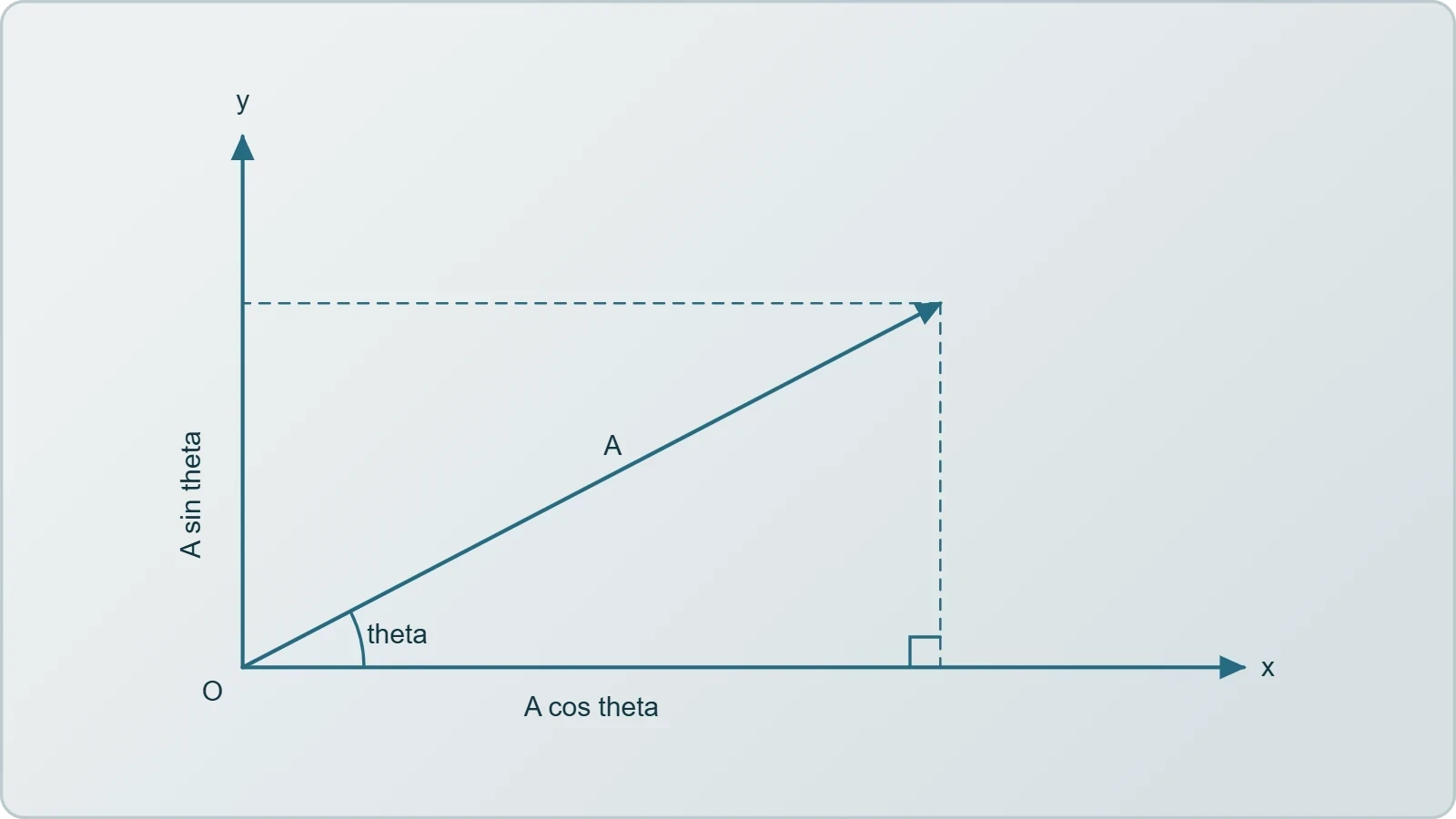
A common examination trap involves quadrant ambiguity: the arctangent function returns values only between ##-90^\circ## and ##+90^\circ##, so a vector pointing into the second or third quadrant requires manual adjustment of the angle. Learners should always sketch the vector before trusting a calculator, since the diagram exposes sign errors that algebra alone conceals.

Vector Addition and the Dot Product

Adding vectors tip-to-tail or by summing components must yield identical results, and checking one method against the other is a powerful self-verification strategy during practice. The dot product, introduced in the previous lesson, extends this toolkit by extracting the component of one vector along another, producing a scalar that encodes alignment.

The dot product's geometric definition, ##\vec{A}\cdot\vec{B} = AB\cos\theta##, connects directly to the component formula ##A_xB_x + A_yB_y##, and reconciling the two expressions is itself an instructive exercise. In planar motion, the dot product answers questions about work done by a force and about whether two velocity vectors are perpendicular at a given instant.

Projectile Motion: Decomposing the Trajectory

Projectile motion rewards learners who trust the independence of horizontal and vertical motion. Once a projectile leaves its launch point, gravity acts only vertically, so the horizontal velocity remains constant while the vertical velocity changes uniformly. This separation transforms an apparently curved path into two straightforward one-dimensional problems solved simultaneously.

Range, Height, and Time of Flight

The standard results for level ground follow from combining the two component equations, and learners should be able to re-derive them rather than merely quote them. Launch speed ##v_0## at angle ##\theta## produces a time of flight, maximum height, and horizontal range that together characterise the entire trajectory.

The range formula reveals a pleasing symmetry: complementary launch angles such as ##30^\circ## and ##60^\circ## produce identical ranges, because ##\sin 2\theta## takes the same value for both. Maximum range occurs at ##45^\circ##, a result worth remembering as a quick sanity check when evaluating numerical answers in practice problems.

Reasoning Beyond the Standard Case

Examination questions rarely stop at level ground, and the review should include projectiles launched from a height or landing on an incline. In such cases the component equations remain valid, but the vertical displacement is no longer zero, so the time of flight must be found by solving a quadratic equation.

Concept questions in this area often probe misconceptions, such as the belief that a faster horizontal launch delays falling. In reality, vertical and horizontal motions are independent, so two balls released simultaneously, one dropped and one projected horizontally, strike the ground at the same instant, neglecting air resistance.

Uniform Circular Motion and Centripetal Acceleration

Circular motion introduces a subtlety that catches many beginners: an object moving at constant speed around a circle is still accelerating, because its velocity vector continuously changes direction. That acceleration points toward the centre of the circle and is called centripetal, meaning centre-seeking. Understanding why it exists, rather than merely memorising its formula, is the goal of this review section.

Speed, Period, and Acceleration

For a body completing a circle of radius ##r## with constant speed ##v##, the period and centripetal acceleration follow from geometry and the definition of acceleration. The derivation uses similar triangles on the velocity vectors, a neat argument worth reconstructing from memory during revision.

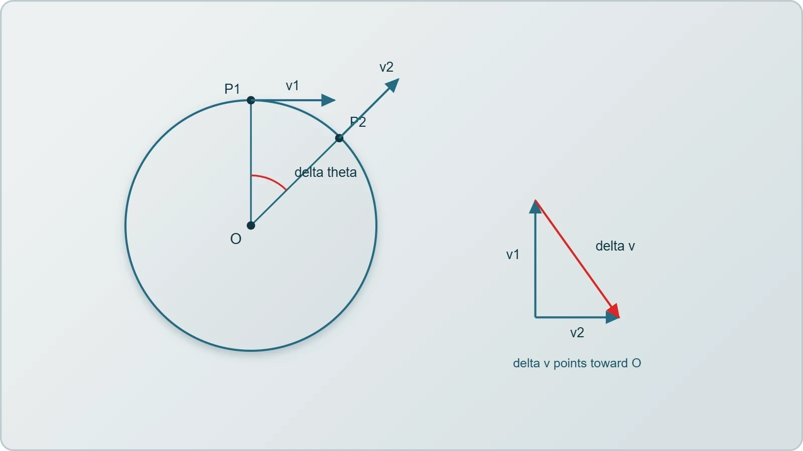
Notice that the acceleration grows with the square of the speed but only inversely with the radius, a relationship that surprises learners who expect larger circles to demand larger accelerations. Practice problems should include both regimes so that the inverse dependence on radius becomes intuitive rather than merely algebraic.

Forces in Circular Paths

Centripetal acceleration must be produced by a real force, whether tension in a string, gravity for a satellite, or friction for a car turning on a road. Concept questions should ask learners to identify the source of the centripetal force in each scenario, since misidentifying it is the most frequent error in this topic.

A persistent misconception holds that a centrifugal force pushes outward; in an inertial frame no such force exists, and the sensation of being flung outward arises from inertia while the actual force points inward. Clarifying this distinction prepares learners for the laboratory experiments that follow, where rotating apparatus makes the effect tangible.

Relative Velocity and Frame Selection

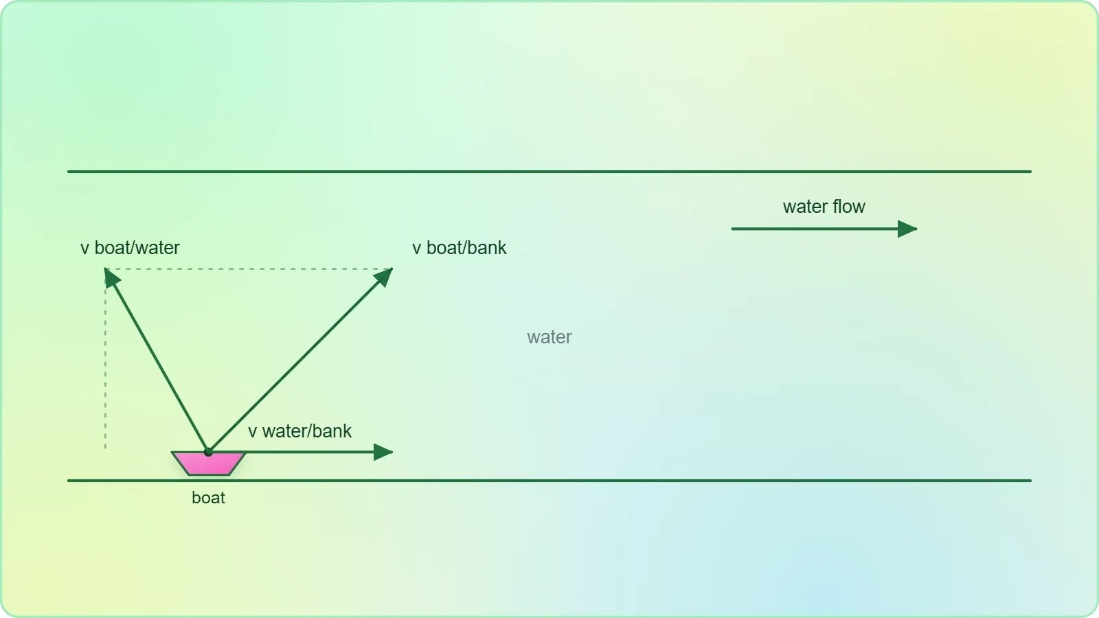
Many planar-motion problems become dramatically simpler when viewed from a cleverly chosen reference frame, and this review should remind learners that velocity is always measured relative to something. A boat crossing a river, an aircraft flying in wind, or a rain drop observed from a moving car all illustrate the same vector-subtraction principle.

The Relative Velocity Equation

The relative velocity of object A with respect to object B is the difference of their velocities measured in a common frame. Applying this relation correctly requires care with signs and with the order of subtraction, since reversing the order reverses the direction of the relative velocity.

River-crossing problems are the classic application: the boat's velocity relative to the water combines with the water's velocity relative to the bank to give the boat's velocity relative to the bank. Learners should practise finding both the minimum crossing time and the heading required to land directly opposite the starting point.

Choosing a Convenient Frame

Frame selection is a strategic skill rather than a formula, and concept questions should reward learners who recognise when a change of frame eliminates complexity. In a collision between two projectiles, for instance, working in the frame of one projectile reduces the problem to straight-line motion of the other.

This idea foreshadows the relativity content that appears in more advanced courses, where the invariance of physical laws across inertial frames becomes a central theme. For now, the practical lesson is that a well-chosen frame converts a tangled two-body problem into a clean one-body problem.

Structured Practice: Worked Problems and Concept Checks

Practice is where review becomes durable learning, and this section models the reasoning expected in a well-argued solution. Each worked example should be read actively: cover the solution, attempt the problem, then compare approaches. The aim is not merely to obtain the right number but to develop a reliable problem-solving routine that transfers to unfamiliar situations.

A Worked Projectile Problem

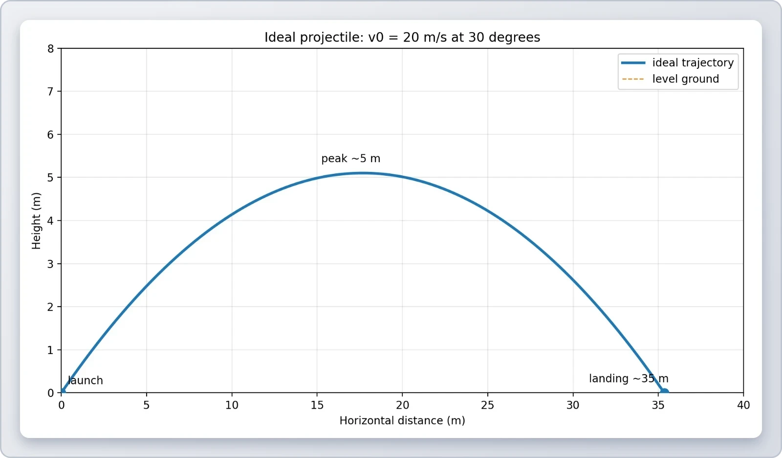
Consider a ball launched at ##20\,\text{m/s}## at ##30^\circ## above the horizontal from level ground, with ##g = 9.8\,\text{m/s}^2##. The vertical component is ##10\,\text{m/s}##, giving a time of flight of roughly ##2.04\,\text{s}## and a range near ##35\,\text{m}##.

Learners should verify each intermediate quantity, check units, and confirm that the answer is physically plausible. A range of thirty-five metres for a twenty-metre-per-second launch is reasonable, and the maximum height of about five metres follows from the vertical component alone.

Concept Questions for Self-Testing

Concept questions probe understanding in ways numerical problems cannot. Why does a projectile's horizontal velocity remain constant? Why does centripetal acceleration not change the speed of a body in uniform circular motion? Answering these aloud, in full sentences, exposes gaps that silent reading conceals.

A useful self-testing routine pairs each formula with a verbal explanation and a limiting case. For instance, the range formula predicts zero range at ##0^\circ## and ##90^\circ##, which matches intuition, and this kind of consistency check builds confidence before examinations and laboratory assessments.

Common Errors and How to Eliminate Them

Most lost marks in planar-motion assessments trace back to a small set of recurring errors, and naming them explicitly is one of the most efficient revision strategies available. Sign mistakes in components, forgotten quadrants, and confusion between speed and velocity account for a surprising share of incorrect answers. A short error audit before each practice session pays immediate dividends.

Diagnosing Frequent Mistakes

Mixing up the sine and cosine in component resolution is common when angles are measured from the vertical rather than the horizontal. Learners should adopt a consistent convention and state it explicitly at the start of every solution, which also makes their reasoning easier for examiners to follow.

Another frequent slip is treating centripetal acceleration as a change in speed rather than direction. Writing a one-line justification beside each circular-motion answer, explaining that the force acts perpendicular to velocity, reinforces the correct conceptual picture and guards against careless errors.

Building Reliable Solution Habits

Reliable habits include drawing a diagram, listing known and unknown quantities with units, choosing equations before substituting numbers, and performing a final plausibility check. These steps cost little time and catch the majority of avoidable mistakes, especially in multi-step projectile problems.

Learners should also practise estimating answers mentally before calculating precisely, since a rough estimate of a few tens of metres for a thrown ball immediately flags a computed range of several kilometres as wrong. Estimation is a skill that laboratory work will demand repeatedly.

Preparing for Laboratory and Real-World Experiments

The next lesson moves from paper problems into physical measurement, and this review closes by bridging the two. In the laboratory, vectors describe forces on a pulley, projectiles leave launchers with imperfect speed, and circular motion appears in rotating platforms. The concepts rehearsed here become instruments for interpreting imperfect data rather than tidy textbook numbers.

From Ideal Models to Measured Reality

Textbook problems neglect air resistance and assume exact launch angles, whereas experiments confront friction, timing uncertainty, and calibration drift. Learners who understand the underlying model can distinguish genuine physical effects from measurement error, which is precisely the judgement laboratory work rewards.

A short code snippet illustrates how a simulation can generate the ideal trajectory that a laboratory experiment then attempts to reproduce, making the comparison between theory and data explicit and quantitative.

import math

def projectile_range(v0, theta_deg, g=9.8):
    theta = math.radians(theta_deg)
    return (v0 ** 2) * math.sin(2 * theta) / g

for angle in (30, 45, 60):
    print(angle, round(projectile_range(20, angle), 2))

Connecting Concepts to Practical Contexts

Real-world applications surround the learner: a basketball shot, a fountain's arc, a car rounding a bend, a satellite in low orbit. Each is a planar-motion problem in disguise, and recognising the underlying structure is the transferable skill this course has been building toward since its first lesson.

Learners preparing for the laboratory should arrive able to predict outcomes, estimate magnitudes, and explain discrepancies in physical terms. That combination of prediction and explanation, rather than formula recall alone, marks the transition from beginner to competent intermediate student of mechanics.