Circular Motion: Non-Uniform Speed

Circular motion rarely behaves with the tidy constancy that introductory physics problems suggest. A ceiling fan spins up from rest, a car eases through a tightening bend, and a roller coaster car sheds speed as it climbs a loop. In each case the object travels a curved path while its speed changes, which means the acceleration vector no longer points neatly toward the centre of the circle. This lesson, the twenty-second in a thirty-part sequence on motion in a plane, isolates that richer situation and gives it a precise mathematical language.

Building directly on the preceding discussion of projectile motion with air resistance, where drag gradually reshapes a trajectory, we now examine how a changing speed reshapes acceleration along a circular path. The central idea is decomposition: acceleration splits into a radial component that bends the velocity and a tangential component that stretches or shrinks it. Mastering this split prepares the ground for the next lesson on relative motion, where observers in different frames disagree about velocities and accelerations.

Expect a treatment grounded in vectors, calculus, and physical intuition rather than memorised formulas. We will derive the tangential acceleration, connect it to angular acceleration, examine the total acceleration vector, and test the ideas against real machinery such as centrifuges and banking roads. By the end, you should be able to look at any curved motion and state, with confidence, exactly which part of the acceleration is turning the object and which part is speeding it up.

From Uniform to Non-Uniform Circular Motion

Uniform circular motion, the comfortable baseline, assumes a constant speed while the direction of velocity rotates steadily. The acceleration then has a single job: to pull the velocity vector around the circle, always pointing toward the centre with magnitude ##a_c = v^2/r##. Nothing in that picture changes the length of the velocity arrow, so the motion never speeds up or slows down.

Non-uniform circular motion relaxes that constraint. The particle still follows a circular path of fixed radius, but the magnitude of its velocity now varies with time. A bead sliding on a vertical wire hoop, a satellite firing thrusters along its orbit, and a washing machine drum during the spin cycle all exhibit this behaviour. The path stays circular; the speed does not.

Why the Acceleration Vector Tilts

When speed changes, a second acceleration component appears along the direction of motion. The radial component continues to handle the turning, while this new tangential component handles the speeding up or slowing down. The total acceleration is their vector sum, and because the two components are perpendicular, the resultant no longer points at the centre of the circle.

This geometric fact carries real consequences. In uniform motion the net force must point radially inward, but in non-uniform motion the net force tilts forward or backward relative to the radius. A car accelerating through a curve therefore needs friction acting at an angle, not purely sideways, which is precisely why tyres squeal more when drivers combine cornering with hard acceleration.

Setting Up the Coordinate Description

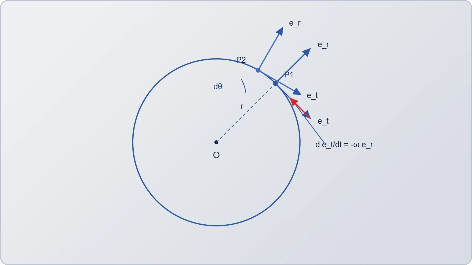
The cleanest description uses a moving frame attached to the particle: a unit vector ##\hat{e}_t## tangent to the path and a unit vector ##\hat{e}_r## pointing radially outward. These basis vectors rotate with the particle, so their own time derivatives are nonzero. That subtlety is the mathematical heart of the topic and the reason calculus earns its place here.

Position on the circle is written as ##\vec{r} = r\hat{e}_r##, with ##r## constant. Differentiating once gives velocity purely along the tangent, and differentiating again produces two terms: one from the changing speed and one from the rotating basis vector. The second term is the familiar centripetal piece; the first is the newcomer we must now examine closely.

Tangential Acceleration and the Rate of Speed Change

Tangential acceleration measures how quickly the speed itself changes, and its definition is disarmingly simple: it equals the time derivative of speed, ##a_t = dv/dt##. Because it lies along the tangent, it does no work in turning the particle; its entire effect is to alter the length of the velocity vector. Positive values mean speeding up, negative values mean slowing down.

This component connects directly to the angular description. Since ##v = r\omega## with ##\omega## the angular speed, differentiating with respect to time yields ##a_t = r\alpha##, where ##\alpha = d\omega/dt## is the angular acceleration. The radius acts as a lever arm, so a point farther from the axis experiences a larger tangential acceleration for the same angular acceleration.

Deriving the Tangential Term from First Principles

Start with the velocity vector expressed in the rotating basis, ##\vec{v} = v\hat{e}_t##. Applying the product rule gives two contributions: one from the changing magnitude ##v## and one from the changing direction of ##\hat{e}_t##. The first contribution is exactly the tangential acceleration, and the second produces the centripetal term.

The rotating basis satisfies ##d\hat{e}_t/dt = -\omega\hat{e}_r##, a relation worth verifying by sketching the vectors at two nearby instants. Substituting this into the derivative of velocity yields the complete acceleration, which we assemble in the next subsection. The derivation rewards patience because every later formula flows from it.

Reading the Two Components Together

The tangential component ##a_t## governs the change in speed, while the radial component ##a_c = v^2/r## governs the change in direction. Their vector sum gives the total acceleration, whose magnitude follows from the Pythagorean relation because the basis vectors are perpendicular. Neither component alone tells the full story of the motion.

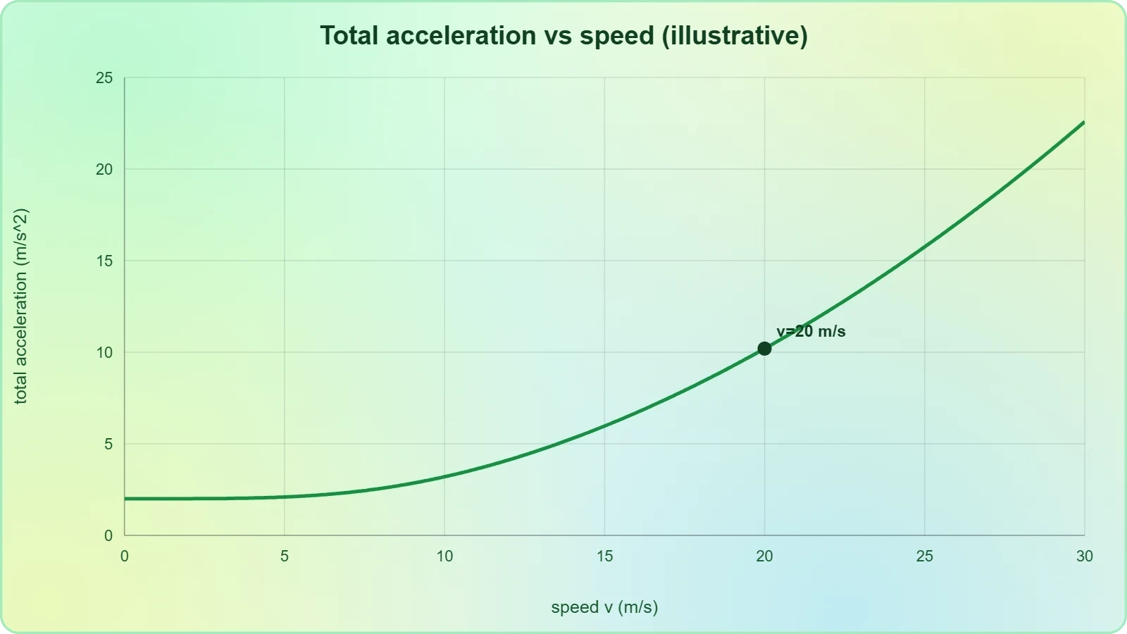
A useful sanity check: when ##a_t = 0##, the total acceleration reduces to the purely radial centripetal form, recovering uniform circular motion as a special case. The general framework therefore contains the simpler one, which is the hallmark of a well-constructed physical theory. Always test new formulas against known limits.

The Total Acceleration Vector and Its Direction

Combining the components produces a total acceleration that points neither purely inward nor purely along the path. Its angle relative to the radius is set by the ratio ##a_t/a_c##, so a gentle speed change yields a vector close to the radial direction, while a violent one tilts it substantially toward the tangent. This angle is the geometric signature of non-uniform motion.

Physically, the net force must align with this total acceleration, since Newton's second law is a vector equation. A particle in non-uniform circular motion therefore requires a force with both radial and tangential parts. Identifying which physical interaction supplies each part is the central analytical skill this lesson develops.

Computing the Angle of the Acceleration Vector

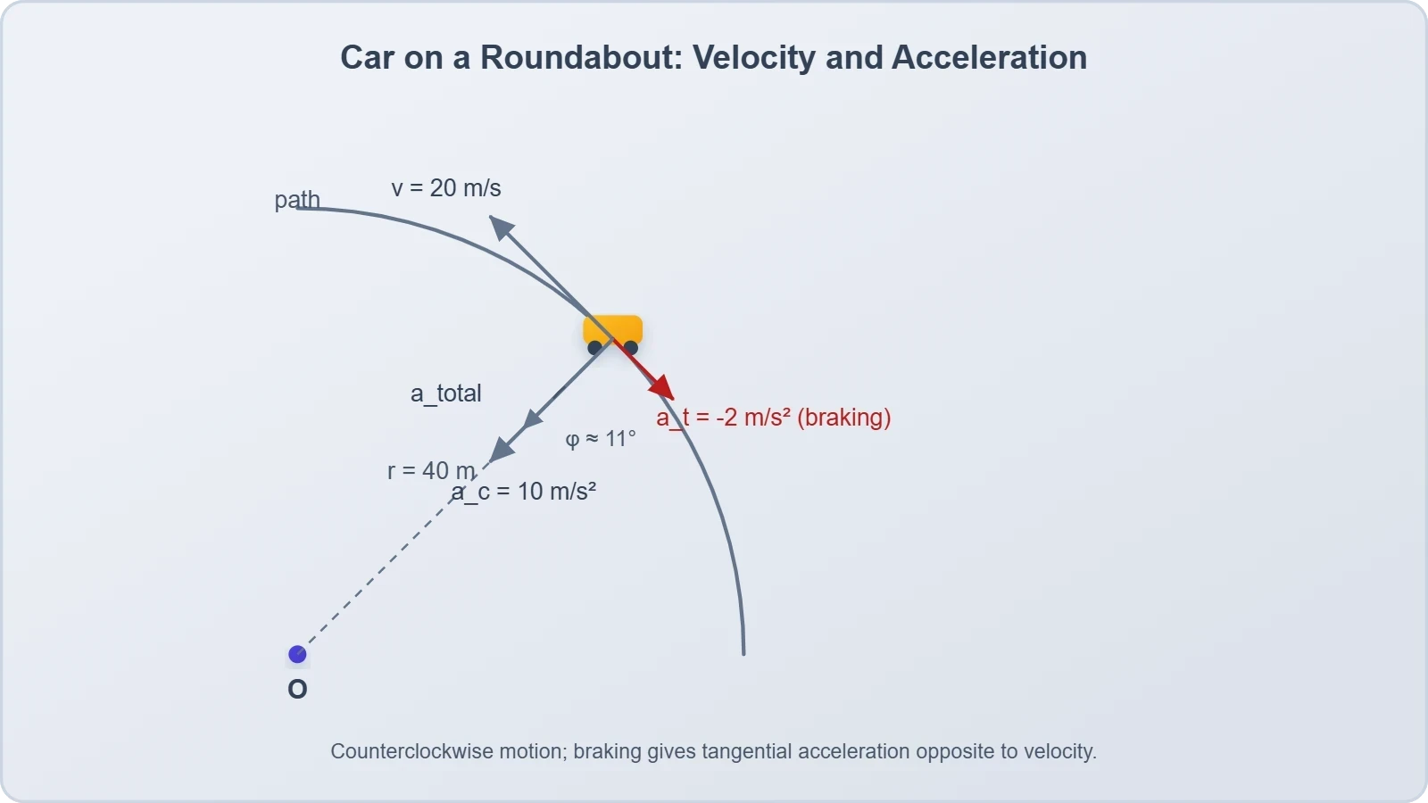
The angle ##\phi## between the total acceleration and the radial direction satisfies ##\tan\phi = a_t/a_c##. Substituting the component formulas gives ##\tan\phi = (dv/dt)/(v^2/r)##, which simplifies to a compact expression involving speed, radius, and the rate of speed change. This single relation summarises the geometry of the motion.

Consider a car entering a roundabout at ##20\,\text{m/s}## on a radius of ##40\,\text{m}## while braking at ##2\,\text{m/s}^2##. The centripetal term is ##10\,\text{m/s}^2## and the tangential term is ##-2\,\text{m/s}^2##, so the acceleration tilts backward by roughly eleven degrees from the radius. The negative sign signals deceleration.

Interpreting the Direction Physically

When the tangential component is positive, the total acceleration leans forward of the radius, meaning the net force pushes the object both inward and ahead. When negative, it leans backward, and the net force opposes the motion while still turning it. The radial part never disappears as long as the object moves on the circle.

This interpretation clarifies everyday experiences. A cyclist leaning into a turn while pedalling hard feels the combined demand on tyre grip, and a roller coaster rider pressed into the seat during a loop senses the changing balance between centripetal and tangential forces. The vector diagram translates directly into bodily sensation.

Angular Kinematics for Changing Speed

When angular acceleration is constant, the angular equations mirror their linear counterparts exactly. Angular velocity evolves as ##\omega = \omega_0 + \alpha t##, angular displacement follows ##\theta = \omega_0 t + \tfrac{1}{2}\alpha t^2##, and a third relation links ##\omega##, ##\alpha##, and ##\theta## without explicit time. These tools handle a large class of practical problems.

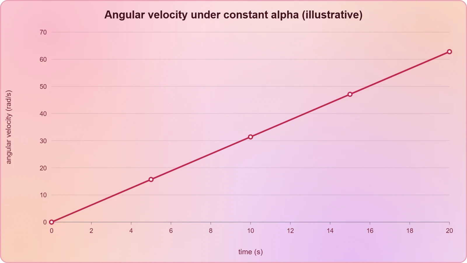
The correspondence is not coincidental; it arises because angular quantities are linear quantities divided by the fixed radius. Every linear kinematic equation therefore has an angular twin obtained by substituting ##s \to \theta##, ##v \to \omega##, and ##a \to \alpha##. Recognising this pattern saves considerable derivation effort and reinforces conceptual unity.

Constant Angular Acceleration in Practice

A centrifuge rotor accelerating uniformly from rest to ##3000\,\text{rev/min}## in twenty seconds illustrates the method. Converting to radians per second and dividing by the time interval yields the angular acceleration, from which the tangential acceleration at the rim follows by multiplying by the radius. The numbers are large, as centrifuges demand.

Such calculations matter in laboratory design, where samples experience enormous effective gravity. A rotor of radius ##0.15\,\text{m}## spinning at ##3000\,\text{rev/min}## produces a centripetal acceleration near ##1.5\times10^4\,\text{m/s}^2##, roughly fifteen hundred times gravity. The tangential term during spin-up is comparatively modest but still significant for mechanical stress.

When Angular Acceleration Varies

If angular acceleration is not constant, the constant-acceleration equations fail and calculus becomes mandatory. One integrates ##\alpha(t)## to obtain ##\omega(t)## and integrates again for ##\theta(t)##. Many real systems, such as motors with load-dependent torque, fall into this category and require numerical or analytical integration.

The following snippet demonstrates a simple numerical integration of variable angular acceleration, a technique useful when no closed-form solution exists. It advances angular velocity and position in small time steps, accumulating the effect of a torque that depends on the current speed. Such simulations underpin engineering analysis of rotating machinery.

import numpy as np

def simulate_rotation(alpha_func, omega0, dt, steps):
    omega = omega0
    theta = 0.0
    history = []
    for _ in range(steps):
        alpha = alpha_func(omega)
        omega += alpha * dt
        theta += omega * dt
        history.append((theta, omega, alpha))
    return history

# Example: angular acceleration decreasing with speed
alpha = lambda w: 2.0 - 0.1 * w
data = simulate_rotation(alpha, omega0=0.0, dt=0.01, steps=1000)
print(data[-1])

Forces, Friction, and Real Rotating Systems

Every acceleration demands a force, and non-uniform circular motion demands two distinct force components. The radial part must supply ##mv^2/r##, while the tangential part must supply ##m\,dv/dt##. In engineered systems these come from different physical sources, and balancing them defines the design envelope of the machine.

For a car on a flat curve, static friction supplies both components, and its maximum value limits the achievable combination of cornering and acceleration. On a banked road, the normal force contributes to the radial requirement, easing the burden on friction. Understanding this division explains why banked tracks allow higher speeds without skidding.

Friction Limits and the Friction Circle

Engineers represent the available friction as a circle in the plane of tangential and radial acceleration. Any demanded acceleration vector must lie inside this circle, or the tyres lose grip. This friction-circle concept, familiar from vehicle dynamics, is a direct application of the vector decomposition developed in this lesson.

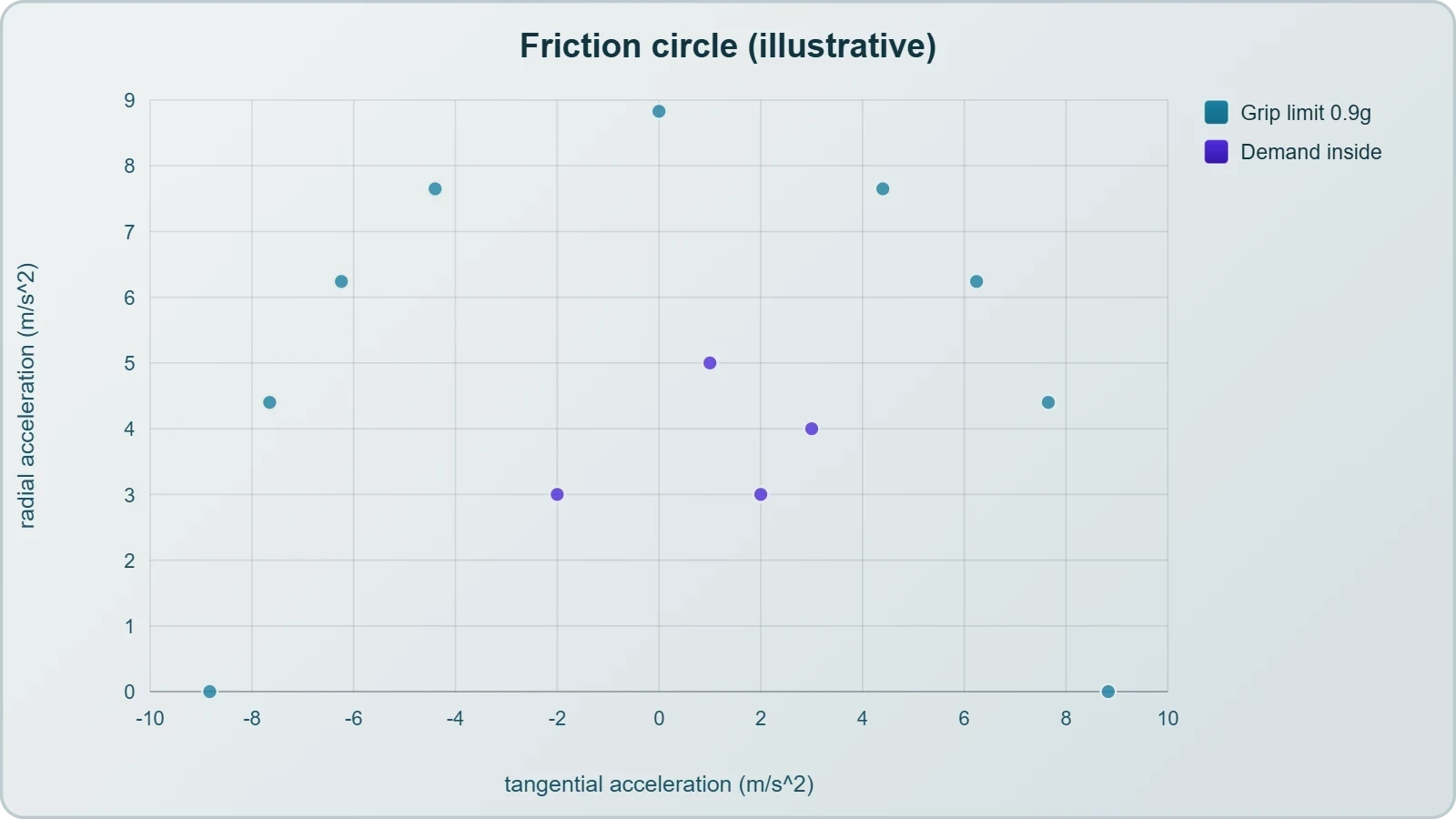
A tyre capable of ##0.9g## total cannot simultaneously deliver ##0.9g## of cornering and ##0.9g## of braking; the vector sum would exceed the limit. Drivers therefore trade cornering against braking, a principle racing engineers exploit when tuning suspension and brake balance for different circuits.

Vertical Circles and Variable Speed

A bead on a vertical hoop experiences gravity as a tangential force that speeds it up on the descent and slows it on the ascent. The radial equation then determines the normal force, which varies around the loop and can vanish at the top if the speed is too low. This classic problem unites both components elegantly.

At the top of the loop, gravity points inward and assists the centripetal requirement, so the normal force may drop to zero at the minimum speed ##v = \sqrt{gr}##. Below that threshold the bead leaves the track. At the bottom, gravity opposes the centripetal demand, and the normal force reaches its maximum.

Problem-Solving Strategy and Common Pitfalls

A reliable procedure begins by drawing the path and marking the instantaneous position, then sketching the tangent and radial directions. Resolve every force along these axes, write the radial equation with ##mv^2/r## on the right, and the tangential equation with ##m\,dv/dt##. Solving the pair yields the unknowns.

Consistency of signs deserves early attention. Choose a positive sense for the tangential direction, usually the direction of motion, and a positive radial sense pointing inward. With those conventions fixed, the algebra proceeds without ambiguity, and the physical meaning of each sign remains transparent throughout the calculation.

Frequent Errors to Avoid

The most common mistake is applying ##v^2/r## with a speed that is changing, treating it as constant over an interval. The formula is instantaneous, so it must be evaluated at the specific moment of interest. Averaging speeds inside it produces incorrect results and muddled reasoning.

Another frequent slip is forgetting that the tangential acceleration changes the speed, which in turn changes the centripetal acceleration. The two components are coupled through ##v##, so a full solution may require integrating the tangential equation before evaluating the radial one. Ignoring this coupling leads to inconsistent answers.

Building Toward Relative Motion

The vector machinery practised here transfers directly to the next lesson, where observers in different frames measure different velocities. The rotating basis vectors introduced in this lesson foreshadow the more general treatment of moving coordinate systems. Each concept now serves as scaffolding for the next.

Before proceeding, verify that you can derive the total acceleration from the position vector, compute the angle of the acceleration, and identify the force sources in a physical system. These competencies form the foundation for relative motion, where the same decomposition reappears in a richer setting.