Projectile Motion with Air Resistance (Qualitative)

Ideal projectile motion, the elegant parabola every beginner learns to sketch, rests on a deliberate fiction: that the air through which the projectile travels exerts no influence whatsoever. In that frictionless dream, horizontal velocity never falters, vertical acceleration stays locked at ##g \approx 9.8\ \text{m/s}^2##, and the trajectory closes into a perfect symmetric arc. Real projectiles, however, move through a fluid that pushes back, and the consequences of that pushback are neither small nor cosmetic. A cricket ball, a badminton shuttlecock, and an artillery shell all trace paths that deviate measurably from the textbook parabola, and understanding why sharpens both physical intuition and practical judgement.

This lesson examines air resistance qualitatively, deliberately postponing the differential equations that would yield exact numerical solutions. The aim is conceptual: to recognise how drag reshapes a trajectory, why the asymmetry between ascent and descent appears, and which physical variables govern the strength of the effect. Building on the problem-solving strategies developed previously, we shift from computing ideal answers to interrogating the assumptions behind them. That habit of questioning idealisations is precisely what prepares a learner for the non-uniform circular motion that follows, where speed itself becomes a variable rather than a constant.

By the end, you should be able to look at any projectile scenario and judge, with sound reasoning, whether the ideal model suffices or whether drag must enter the analysis. You will also appreciate why engineers designing parachutes, golf balls, and aircraft approach the same physics from opposite directions, sometimes minimising drag and sometimes exploiting it. The mathematics remains light, but the conceptual payoff is substantial.

The Ideal Parabola and Its Hidden Assumptions

Before confronting drag, we must be precise about what the ideal model actually claims. The standard treatment decomposes motion into independent horizontal and vertical components, with the horizontal velocity constant and the vertical motion governed solely by gravity. Every textbook derivation of range, maximum height, and time of flight flows from these two premises, and every one of them quietly assumes a vacuum.

Decomposing Motion Without Resistance

In the ideal case, the horizontal equation of motion is trivially ##v_x = u_x##, a constant, because no horizontal force exists. The vertical equation reads ##v_y = u_y - gt##, a linear decline in upward speed until the projectile reverses direction. Combining these gives the familiar parabolic trajectory, whose symmetry about the apex is a direct consequence of gravity being the only acceleration present.

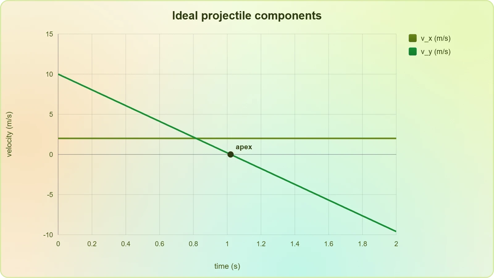
This decomposition is powerful because it isolates two independent one-dimensional problems. The horizontal problem is trivial, the vertical problem is uniformly accelerated motion, and the two recombine through the shared time variable ##t##. Recognising that the symmetry of the parabola depends entirely on the absence of horizontal forces is the first step toward understanding what drag destroys.

Why the Vacuum Assumption Rarely Holds

Air at sea level has a density near ##1.2\ \text{kg/m}^3##, and any object moving through it collides with countless molecules every second. For slow, dense, compact objects the resulting force is negligible; for fast, light, or large-surface-area objects it dominates. The vacuum assumption is therefore not wrong in principle but conditional in practice, valid only within a regime defined by the object and its speed.

This conditional validity is a recurring theme in physics education. Models are tools with domains of applicability, and a competent physicist always asks whether the current situation lies inside or outside that domain. Projectile motion with air resistance is an ideal vehicle for cultivating that professional scepticism.

The Nature of Drag Forces

Air resistance is not a single phenomenon but a family of effects whose relative importance shifts with speed, size, and shape. At low speeds, the air flows smoothly around the object and the resistance arises from viscous shearing within the fluid; at high speeds, turbulence and pressure differences dominate. Both regimes produce a force opposing motion, but their scaling with velocity differs fundamentally, and that difference has visible consequences for trajectories.

Linear and Quadratic Drag Regimes

At low Reynolds numbers, drag is approximately proportional to velocity, giving ##\vec{F}_d = -b\vec{v}## for some constant ##b##. At higher speeds, the force scales with the square of speed, ##\vec{F}_d = -\tfrac{1}{2}\rho C_d A v^2 \hat{v}##, where ##\rho## is air density, ##C_d## the drag coefficient, and ##A## the cross-sectional area. Most everyday projectiles, from thrown stones to struck balls, inhabit the quadratic regime.

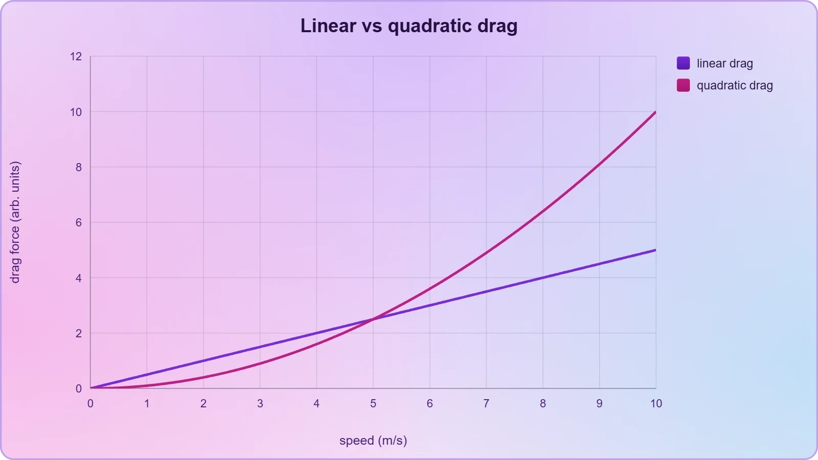
The quadratic dependence is the crucial qualitative fact. Doubling the speed quadruples the drag, so fast projectiles suffer disproportionately. This nonlinearity is precisely what makes the resulting motion analytically intractable and what produces the dramatic departures from parabolic form that we now examine.

Dependence on Shape, Size, and Speed

The drag coefficient ##C_d## encodes shape: a streamlined teardrop may have ##C_d \approx 0.04##, while a flat plate presents roughly ##1.2##. Cross-sectional area enters linearly, so a large light object such as a shuttlecock experiences enormous deceleration relative to its weight. Mass matters too, since a heavier object of identical shape resists the same drag force more effectively.

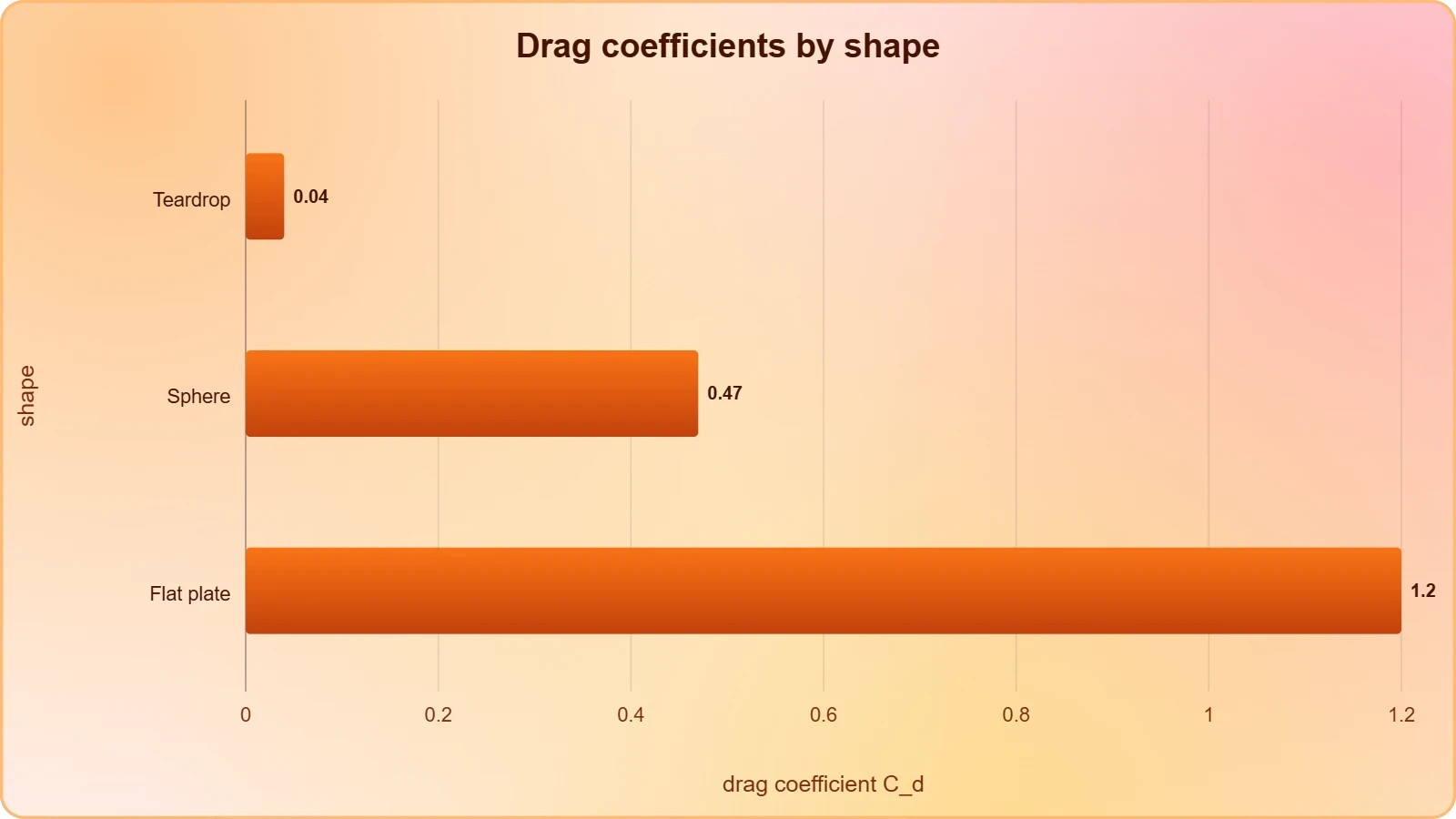
These dependencies explain the familiar observation that a feather and a hammer behave utterly differently in air yet identically in vacuum. The ratio of drag force to weight, not the drag force alone, governs the visible deviation from ideal motion. This ratio is the single most useful diagnostic for judging whether air resistance matters in a given scenario.

How Drag Reshapes the Trajectory

Introducing drag breaks the symmetry that defines the ideal parabola, and the breakage is systematic rather than random. The trajectory becomes skewed, the apex shifts, the range contracts, and the descent steepens relative to the ascent. Each of these distortions can be traced to a single cause: the drag force always opposes the instantaneous velocity, so it acts differently on the way up than on the way down.

Asymmetric Ascent and Descent

During ascent, velocity has an upward component, so drag points partly downward, reinforcing gravity and decelerating the projectile more sharply than ##g## alone would. The projectile therefore rises less far and for less time than the ideal model predicts. At the apex, where vertical velocity vanishes, drag acts purely horizontally, and the horizontal speed has already been eroded throughout the climb.

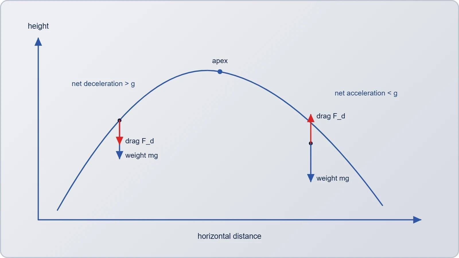
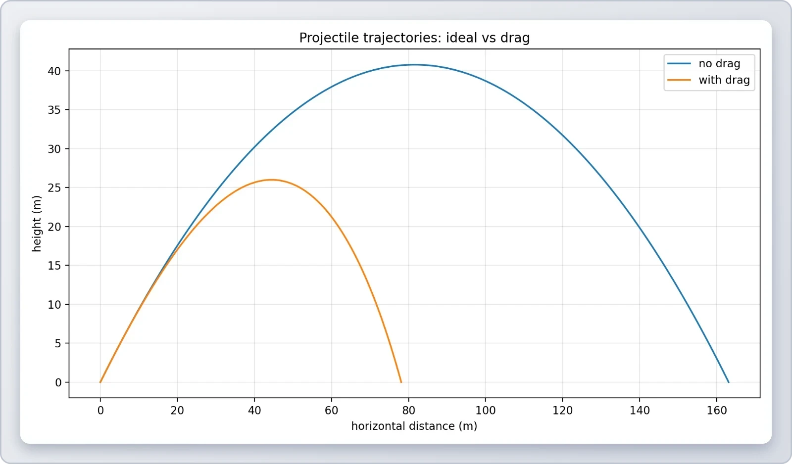
During descent, velocity points downward, so drag now opposes gravity, reducing the net downward acceleration below ##g##. The projectile falls more slowly than free fall would dictate, yet because it has lost horizontal speed, the descent path is steeper. The result is a trajectory whose descending branch is noticeably more vertical than its ascending branch, a signature asymmetry absent from the ideal parabola.

Reduced Range and Shifted Apex

The cumulative effect on range is severe. For a golf ball driven at typical speeds, drag can cut the ideal range by more than half, which is why real golf balls are dimpled to manage boundary-layer behaviour and partially recover distance. The apex, meanwhile, occurs earlier and lower than the symmetric model predicts, since the ascent is curtailed.

These shifts matter practically. Artillery tables, sporting trajectories, and even water-jet fountain designs must account for them, often through empirical correction rather than closed-form solution. The qualitative lesson is robust: drag always shortens range and lowers the apex for a given launch speed and angle.

Terminal Velocity and the Limits of Falling

When an object falls far enough, drag grows with speed until it balances weight exactly, and acceleration ceases. This equilibrium speed, the terminal velocity, is a direct and observable consequence of quadratic drag, and it caps the speed any falling body can attain in a fluid. The concept bridges projectile motion and the broader study of motion through resistive media.

Balancing Weight Against Drag

Setting drag equal to weight gives ##\tfrac{1}{2}\rho C_d A v_t^2 = mg##, which rearranges to ##v_t = \sqrt{2mg/(\rho C_d A)}##. The formula shows that terminal velocity rises with mass and falls with area and drag coefficient, explaining why a skydiver spreads limbs to slow the fall and tucks to accelerate.

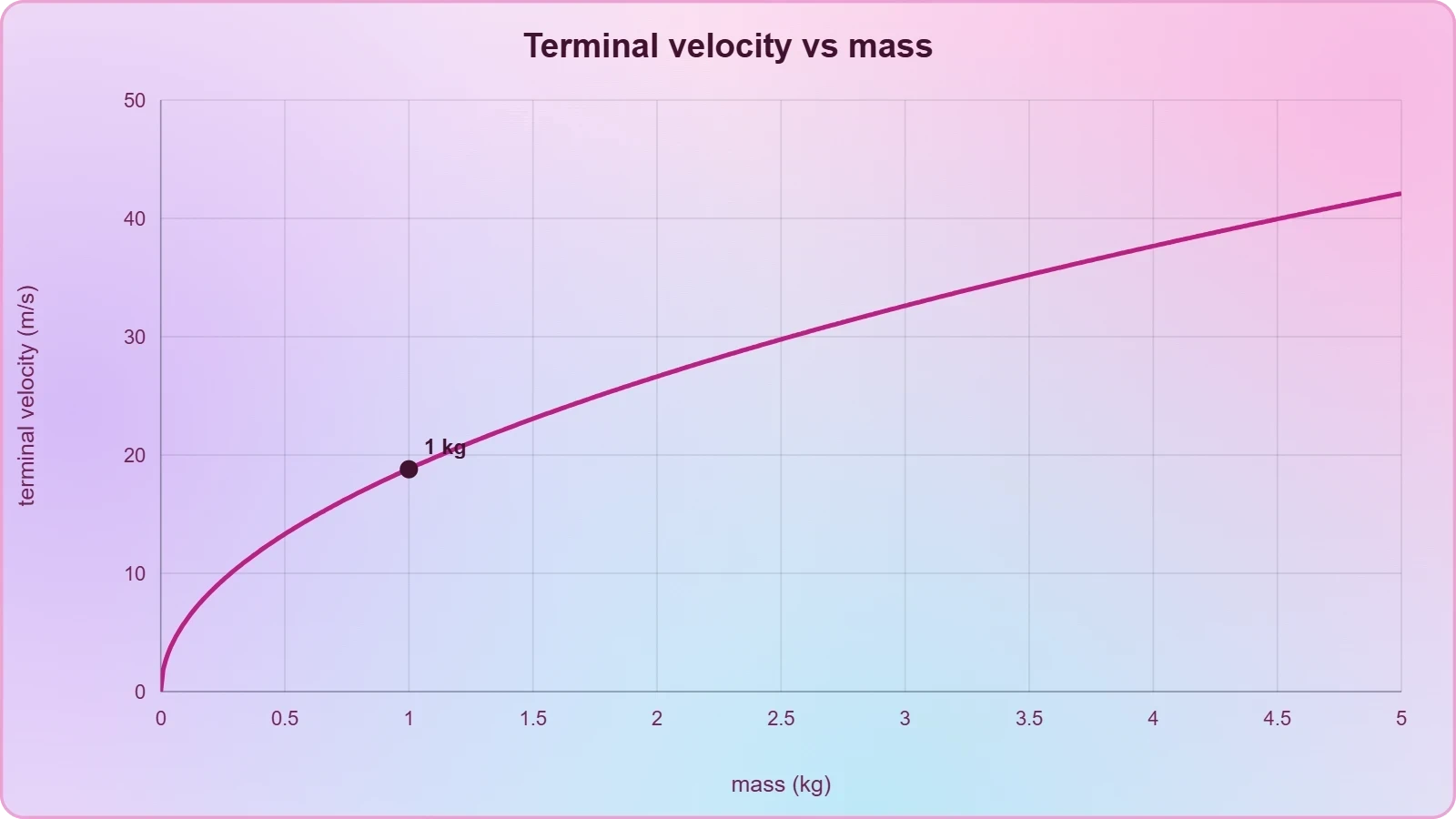
For a human in free fall, terminal velocity is roughly ##50\ \text{m/s}## in a spread posture and considerably higher when streamlined. Raindrops, by contrast, reach only a few metres per second, which is why they arrive as gentle droplets rather than lethal pellets. The formula is a compact illustration of how geometry and mass conspire.

Why Projectiles Never Truly Follow Parabolas

Strictly speaking, no projectile in air follows a parabola, because the drag force depends on velocity and therefore changes continuously along the path. The parabola is a limiting case approached only as drag vanishes, and the terminal velocity marks the extreme where the trajectory becomes almost vertical and speed saturates.

This recognition reframes the ideal model as an approximation with a measurable error, not a truth. The professional habit is to estimate that error before trusting the ideal result, asking whether the projectile's speed is small compared with its terminal velocity. If it is, the parabola serves well; if not, qualitative corrections are mandatory.

Launch Angle and the Optimal Trajectory

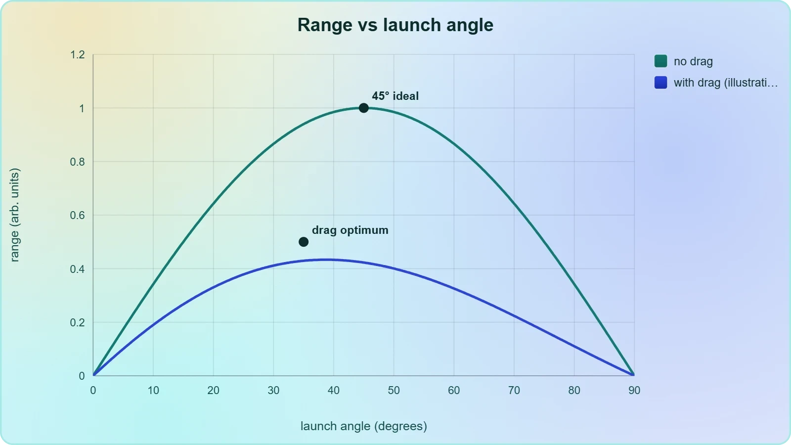
In a vacuum, the range of a projectile launched and landing at the same height is maximised at exactly ##45^\circ##, a result that follows cleanly from the range formula ##R = u^2\sin 2\theta / g##. With drag present, this elegant result fails, and the optimal angle drops below forty-five degrees. The shift is small but real, and it carries instructive lessons about how idealisations mislead.

Why Forty-Five Degrees Fails

A steeper launch spends more time aloft, and drag acts throughout that time, eroding horizontal speed relentlessly. A shallower launch reduces flight time and thus the total drag impulse, trading height for preserved horizontal velocity. The optimum therefore tilts toward lower angles, typically in the range of ##30^\circ## to ##40^\circ## depending on the drag strength.

This is a qualitative insight worth internalising: when a dissipative force acts, the strategy that maximises a quantity in the ideal case is rarely optimal in reality. The same logic appears in optics, where the path of least time differs from the straight line, and in economics, where frictionless models misprice risk.

Practical Consequences for Sport and Engineering

Golfers, javelin throwers, and artillery officers all confront this shift empirically. The javelin's optimal release angle is well below forty-five degrees, and shot-putters exploit similar corrections. Engineers designing projectiles use numerical integration of the drag equations rather than closed-form formulas, precisely because the analytic ideal is inadequate.

The lesson generalises beyond sport. Any engineering domain where a resistive force scales with speed must treat the ideal optimum as a starting point, not an answer. The professional instinct is to ask how far reality departs from the ideal and whether that departure is tolerable.

Judging When Air Resistance Matters

The central practical skill of this lesson is the ability to decide, quickly and defensibly, whether a given projectile problem demands drag corrections. The decision rests on comparing the drag force at typical speeds with the projectile's weight, and on estimating whether the resulting deviation exceeds the precision required. This is engineering judgement, not pure mathematics.

The Drag-to-Weight Ratio as a Diagnostic

If the drag force at launch speed is a small fraction of the weight, the ideal parabola is an excellent approximation. If it approaches or exceeds the weight, the trajectory will be visibly distorted. The ratio ##F_d/(mg)## therefore serves as a single dimensionless number summarising the importance of air resistance for a given scenario.

Computing this ratio requires only the drag formula and the object's mass, both readily available. A steel ball bearing and a beach ball of similar size differ enormously in this ratio, and their trajectories differ correspondingly. The diagnostic converts a vague worry about air resistance into a concrete, checkable calculation.

Choosing the Right Model for the Problem

Once the ratio is known, model selection follows naturally. Small ratio, use the ideal equations and quote the approximation. Large ratio, either integrate numerically or reason qualitatively about the direction of the corrections. The professional never applies the ideal model blindly, nor abandons it needlessly.

This disciplined approach to modelling is the deeper lesson of the lesson. Physics advances by knowing which complications can be safely ignored and which cannot, and projectile motion with air resistance is a compact training ground for that judgement. The next lesson, on non-uniform circular motion, extends the same reasoning to a new geometry.

From Qualitative Insight to Numerical Practice

Qualitative reasoning establishes the direction and rough magnitude of drag effects, but engineering practice ultimately demands numbers. Numerical integration of the equations of motion, with drag included, is straightforward and reveals the full trajectory. A brief exposure to the method consolidates the qualitative lessons and prepares learners for computational work later in their studies.

A Simple Numerical Integration Sketch

The idea is to advance the projectile in small time steps, updating velocity from the net force and position from the velocity. Drag is recomputed at each step from the current velocity, so the nonlinearity is handled naturally. The following Python sketch illustrates the structure without claiming high accuracy.

import math

g = 9.81
rho = 1.2
Cd = 0.47
radius = 0.11
mass = 0.43
area = math.pi * radius**2

def simulate(vx, vy, dt=0.001):
    x, y = 0.0, 0.0
    while y >= 0:
        v = math.hypot(vx, vy)
        drag = 0.5 * rho * Cd * area * v
        ax = -drag * vx / mass
        ay = -g - drag * vy / mass
        vx += ax * dt
        vy += ay * dt
        x += vx * dt
        y += vy * dt
    return x

print(simulate(20.0, 20.0))

Running such a simulation with and without the drag term makes the qualitative predictions concrete: the range shrinks, the apex lowers, and the descent steepens. The code is deliberately simple, but it embodies the professional method of replacing an intractable analytic problem with a tractable numerical one.

Connecting to the Next Lesson

The reasoning developed here, comparing forces, questioning idealisations, and choosing models by regime, transfers directly to circular motion at non-uniform speed. There, tangential acceleration joins centripetal acceleration, and the same discipline of separating ideal from real applies. The conceptual toolkit assembled in this lesson will be reused immediately.

Learners should leave with a durable habit: never accept a parabolic trajectory without asking what the air is doing. That single question, asked routinely, distinguishes a careful physicist from a formula-reciting one. The mathematics of drag can wait; the judgement cannot.