Vectors in Real-World Contexts

Vectors rarely announce themselves as vectors. A pilot trimming a heading against a crosswind, a sailor tacking up an estuary, a goalkeeper reading the flight of a curling free kick, and a structural engineer resolving cable tensions on a suspension bridge are all performing the same quiet arithmetic: decomposing a slanted quantity into perpendicular parts, then recombining them into a single meaningful result. Lesson 19 of this course takes the formal machinery built across the preceding eighteen lessons and places it squarely in the physical world, where arrows on paper become forces on steel, currents in water, and velocities in open air.

The organising idea is transfer. Having established in the previous lesson how to read motion in a plane from graphs, learners now confront situations where the graph is absent and the geometry must be constructed from the scenario itself. Navigation supplies the cleanest entry point because headings, bearings, and drift are naturally vector quantities with immediate visual meaning. Sport adds the complication of spin, bounce, and human timing. Engineering closes the loop by demanding precision, since a misresolved force component in a truss or a crane rig carries consequences measured in tonnes rather than marks.

Throughout, the treatment remains deliberately applied rather than abstract. Every worked example begins with a described situation, proceeds through a labelled vector diagram, and ends with a numerical answer whose plausibility can be judged against common sense. The lesson also prepares the ground for the problem-solving strategies that follow, since real contexts are precisely where the choice of coordinate axes, the decision to resolve or to use the cosine rule, and the discipline of tracking units begin to matter most.

Why Real Contexts Change How Vectors Behave

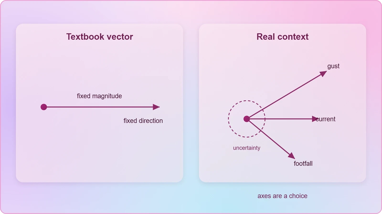
Textbook vectors arrive pre-labelled, neatly orthogonal, and conveniently free of friction. Real contexts refuse that courtesy. Wind gusts vary with altitude, river currents slow near the banks, and a sprinter's acceleration changes with every footfall, so the vector model becomes an approximation chosen for usefulness rather than a perfect description of nature. Recognising which simplifications are legitimate is itself a core skill of applied kinematics.

From Diagram to Decision

The decisive shift is that a vector diagram in a real context must be defended. Choosing north as the reference axis is a convention, not a law, and a navigator may equally choose the direction of travel or the runway centreline. The physics is invariant under that choice, but the arithmetic is not equally convenient, and experienced practitioners select axes that minimise the number of components requiring resolution.

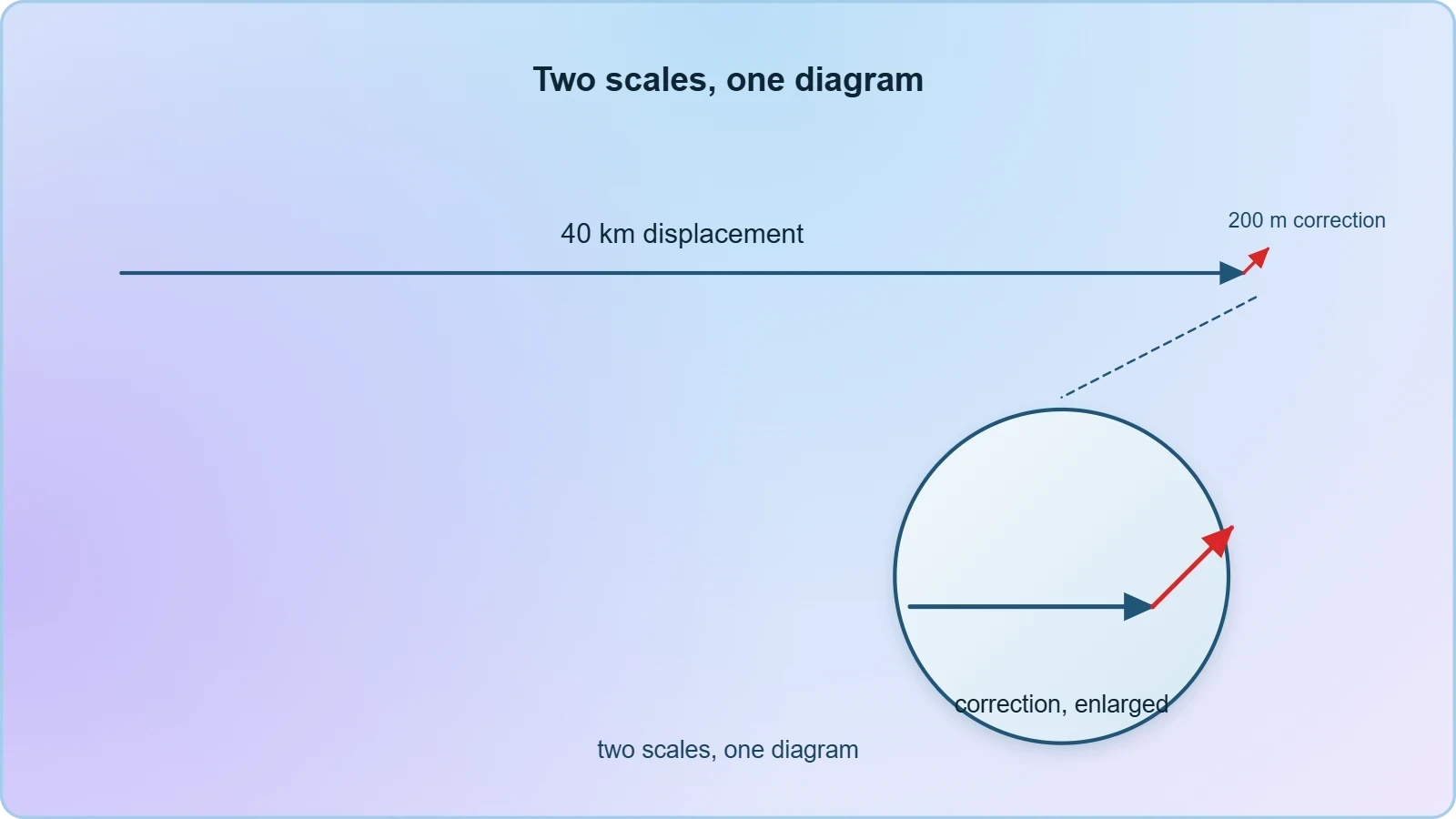
Equally important is the question of scale and tolerance. A displacement vector drawn to represent forty kilometres cannot show a two-hundred-metre correction, yet that correction may be the entire point of the exercise. Applied vector work therefore separates the strategic diagram, which shows directions and relationships, from the numerical calculation, which carries the precision.

Scalars That Hide Inside Vectors

Speed, distance, and time are scalars, yet they interlock with vector quantities in ways that trip the unwary. A vessel may travel thirty nautical miles through the water while its displacement over ground is only twenty-two, because the water itself moved. Distinguishing path length from displacement magnitude is not pedantry; it is the difference between a fuel calculation that works and one that strands the boat.

The same distinction governs athletic performance. A footballer sprinting a curved forty-metre run covers forty metres of ground but registers a much smaller displacement, and the direction of that displacement determines whether the run was tactically useful. Coaches increasingly use this vector reasoning, alongside GPS vests, to evaluate movement efficiency rather than raw distance covered.

Navigation: Bearings, Drift, and the Triangle of Velocities

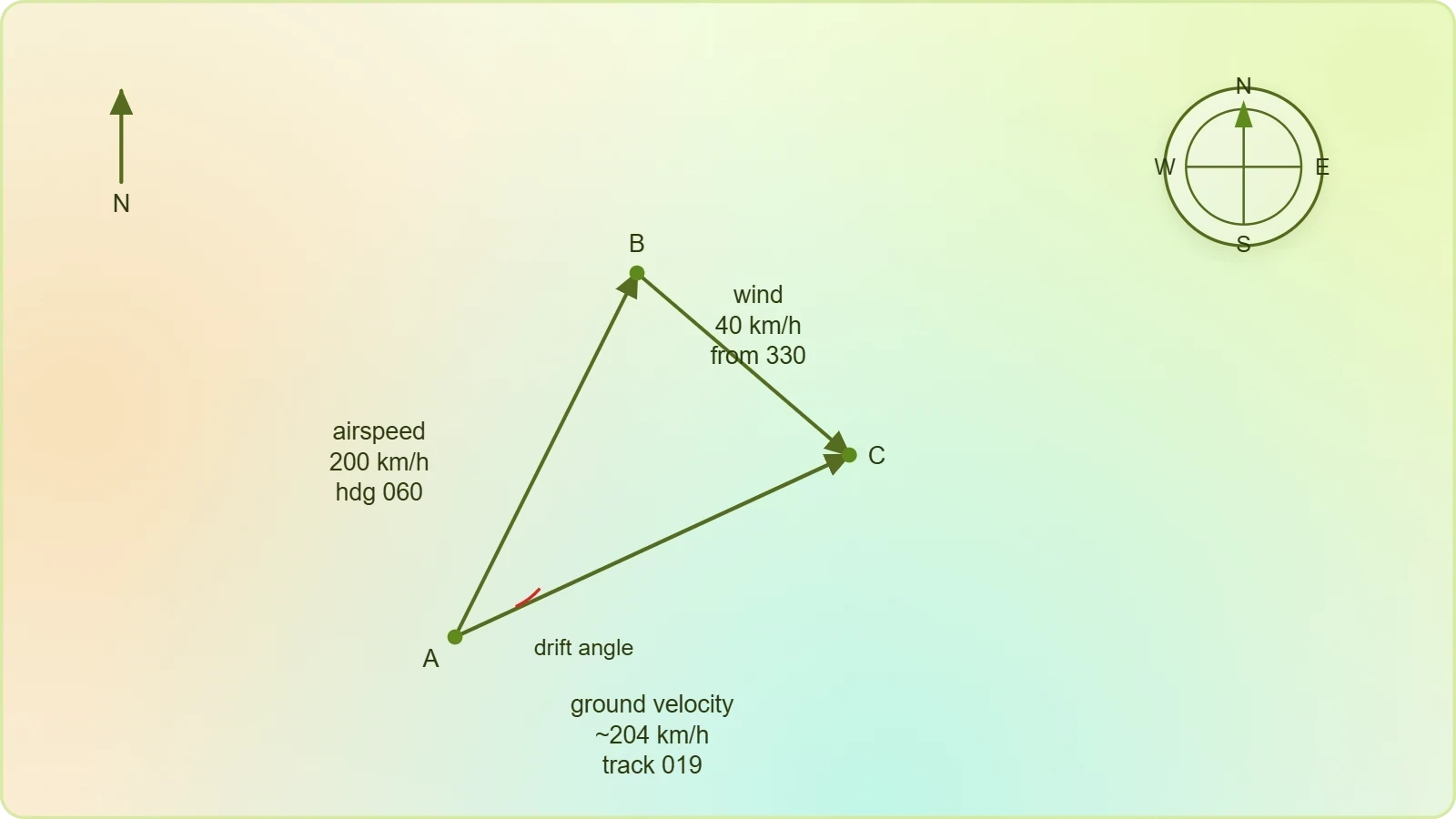
Navigation is vector addition made compulsory. An aircraft's velocity relative to the air is one arrow; the wind's velocity relative to the ground is a second; the aircraft's velocity relative to the ground is their sum. Because the three form a closed triangle, any two determine the third, which is why pilots, mariners, and drone operators all solve the same triangle with different instruments.

Working the Wind Triangle

Suppose an aircraft flies with airspeed ##v_a = 200\ \text{km/h}## on a heading of ##060^\circ## while a wind of ##w = 40\ \text{km/h}## blows from ##330^\circ##. Resolving both into east and north components and adding them yields the ground velocity, whose magnitude and bearing follow from Pythagoras and the tangent ratio. The drift angle is the angular gap between heading and track.

The correction is then applied in reverse: to hold a desired track, the pilot steers into the wind by the drift angle, and the resulting ground speed differs from the airspeed. This iterative reasoning, familiar to every flight-planning student, is nothing more than the vector equation below, solved for the unknown heading.

Mariners face the identical structure with tide replacing wind, and the stakes are tangible: a ferry crossing a tidal estuary must aim upstream by an angle whose sine is the ratio of current speed to boat speed. Failure to do so produces a curved track and a longer crossing, a phenomenon every harbour pilot accounts for as a matter of routine.

Bearings, Conventions, and Sign Discipline

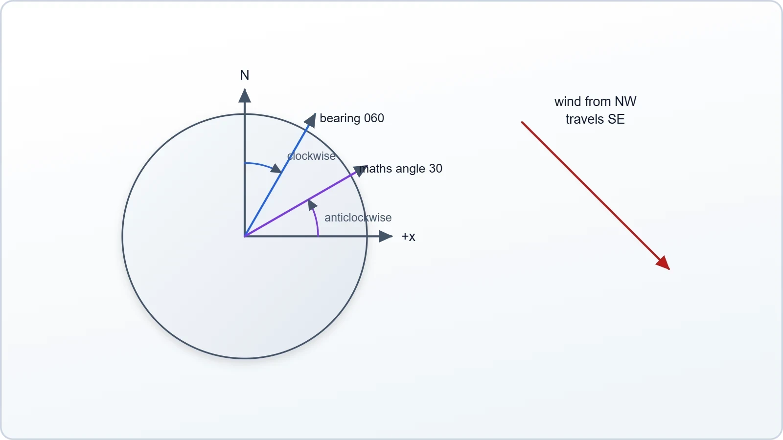
Bearings are measured clockwise from north, whereas mathematical angles are measured anticlockwise from the positive x-axis. Mixing the two conventions is the single most frequent error in navigation problems, and the remedy is to convert everything to one system before resolving any component. A sketch with a compass rose prevents most of these slips.

Sign discipline extends to the components themselves. A wind from the north-west blows towards the south-east, so its velocity vector points opposite to its name. Learners who record the direction of origin rather than the direction of travel will produce a triangle that closes but answers the wrong question, a mistake worth anticipating explicitly.

Sport: Projectiles, Spin, and the Geometry of Timing

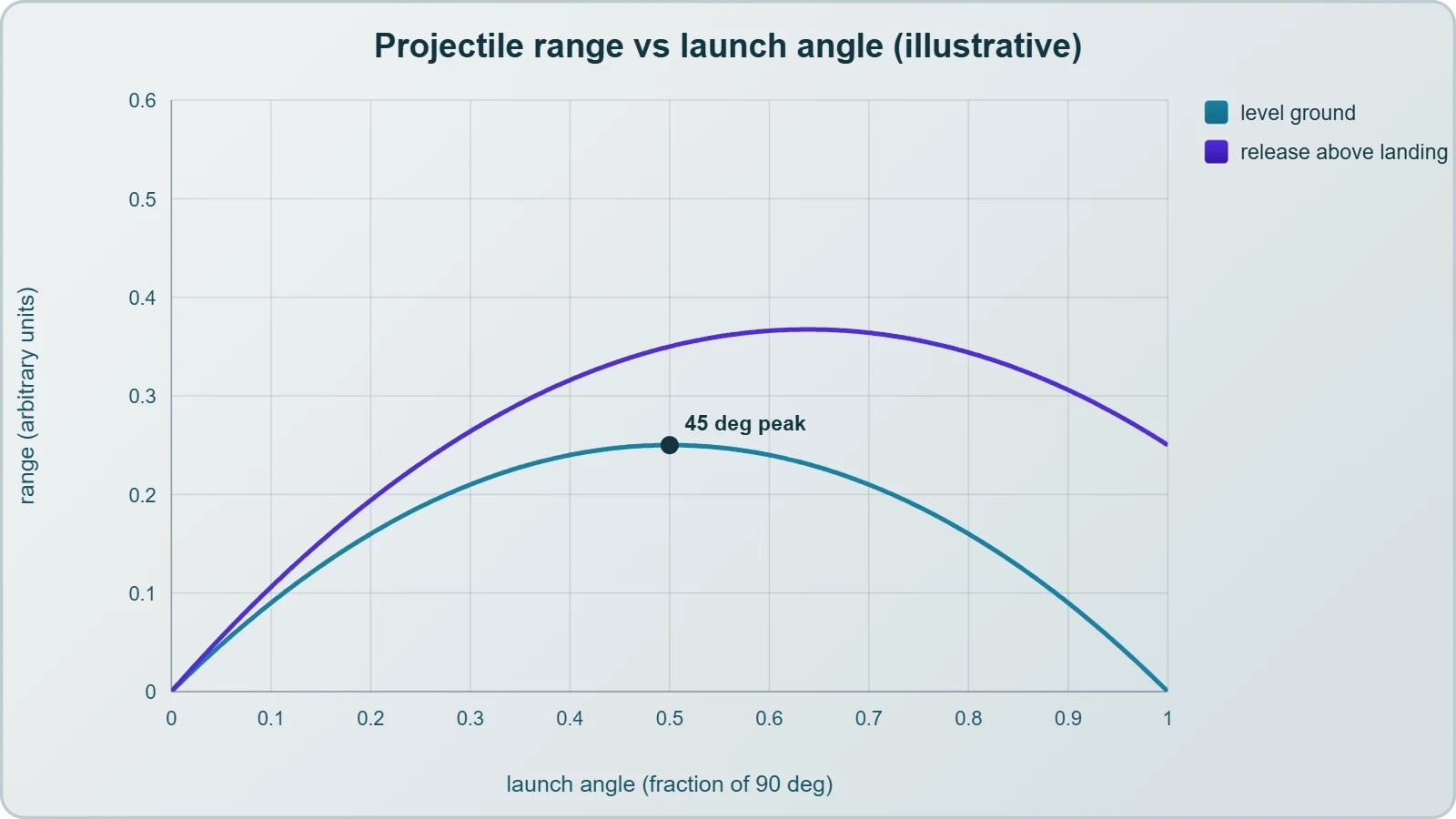
Athletic contests are vector problems with spectators. A long jumper's optimum take-off angle is not the textbook forty-five degrees, because the jumper's centre of mass begins and ends at different heights and the run-up speed constrains what is achievable. Coaches therefore treat the projectile equations as a family of trade-offs rather than a single formula to be memorised.

Range, Release Height, and the Real Optimum

For a projectile launched and landing at the same height, range is maximised at ##45^\circ##. When release occurs above landing height, as in shot put or the javelin, the optimum angle falls below forty-five degrees, and the heavier the implement the more the athlete's strength limits the achievable speed. The mathematics explains why elite throwers release flatter than intuition suggests.

This expression assumes level ground and negligible air resistance, and both assumptions deserve scrutiny. Drag reduces range and shifts the optimum angle downward, while a tailwind extends it. The equation is therefore a baseline against which real performances are interpreted, not a prediction of them.

Curling Balls, Spinning Balls, and Deflection

When a ball spins, the air pressure on one side differs from the other, producing a lateral force perpendicular to the velocity. The result is the banana free kick, the swinging cricket delivery, and the curving tennis serve. The deflection is a vector perpendicular to motion, so the trajectory bends continuously rather than simply slowing.

Players exploit this deliberately. A footballer striking the ball off-centre imparts spin whose axis determines the direction of curve, and the goalkeeper must predict a path that is not a parabola. The vector reasoning is identical to the wind triangle, except the deflecting influence arises from the ball's own rotation rather than the surrounding air mass.

Engineering: Resolving Forces in Structures and Machines

Engineering converts vector reasoning into safety margins. A suspension bridge cable carries tension along its own axis, a truss member carries force along its length, and a crane sling carries load in two directions at once. In each case the analysis begins by resolving forces into components and demanding that the sums vanish where the structure is at rest.

Equilibrium and the Free-Body Diagram

The condition for static equilibrium in a plane is deceptively compact: the sum of all force components in each direction must be zero. Written formally, ##\sum F_x = 0## and ##\sum F_y = 0##, with a third condition on moments if the body can rotate. Every statics problem reduces to applying these statements to a carefully drawn free-body diagram.

Consider a sign of weight ##W## hanging from two cables inclined at ##30^\circ## and ##60^\circ## to the horizontal. Resolving horizontally shows the tensions are unequal; resolving vertically fixes their magnitudes. The steeper cable carries the larger share, a result that surprises learners until they recognise that the steeper cable supports more of the vertical load.

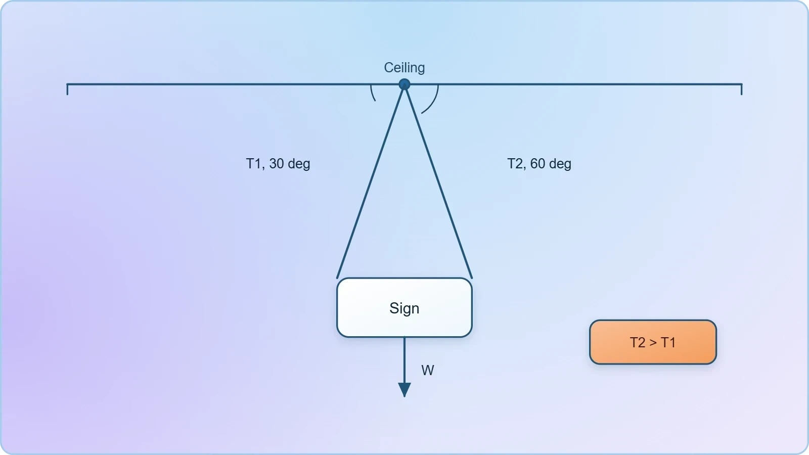
This pair of equations is the workhorse of introductory statics, and its structure recurs in roof trusses, cable-stayed masts, and the rigging of sailing yachts. The mathematics does not care whether the structure is a bridge or a mast; only the geometry of the angles changes.

Relative Velocity in Machinery and Traffic

Relative velocity appears wherever two moving bodies must be compared. A conveyor belt carrying packages, a robotic arm tracking a part, and two vehicles approaching a junction all require the velocity of one body as measured from the other. The rule is simple subtraction of vectors, but its consequences are not always intuitive.

Two cars approaching at right angles each at ##60\ \text{km/h}## have a relative speed of ##60\sqrt{2} \approx 85\ \text{km/h}##, not zero and not one hundred and twenty. Traffic engineers use exactly this reasoning when setting sight-line distances at junctions, since the closing speed determines the time available for a driver to react.

Circular Motion in Practice: Rotors, Rides, and Roadways

Uniform circular motion appears wherever something turns steadily: a centrifuge, a fairground ride, a car on a bend, a satellite in low orbit. The velocity is tangential and constantly changing direction, so an inward acceleration exists even when speed is constant. Its magnitude is ##a = v^2/r##, directed towards the centre of the circular path.

Banked Curves and Design Speed

Road designers bank curves so that the horizontal component of the normal reaction supplies the required centripetal force. At the design speed, no friction is needed at all, which is why racing circuits and motorway bends are engineered around a specific velocity. The relationship below defines that ideal condition.

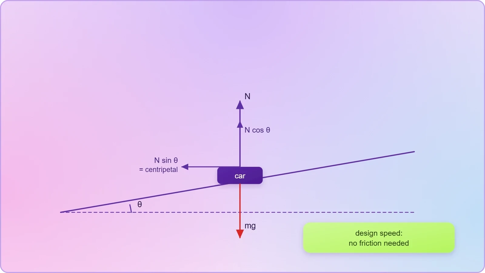
Below the design speed, friction acts up the slope to prevent sliding down; above it, friction must act down the slope to prevent sliding out. The same equation governs the tilt of a velodrome track and the banking of railway curves, where the outer rail is raised by a carefully calculated amount.

Centrifuges and Apparent Weight

A centrifuge exploits the same physics in reverse, spinning samples so that the required centripetal acceleration is many times ##g##. At ##10{,}000## revolutions per minute with a rotor radius of ##0.1\ \text{m}##, the acceleration reaches roughly ##1.1\times10^{4}\ \text{m/s}^2##, over a thousand times gravity, which separates components of differing density with remarkable speed.

Astronauts experience an analogous effect during launch and re-entry, where sustained acceleration vectors combine with gravity to produce a felt resultant. The discomfort is not a mysterious force but the vector sum of real accelerations, and understanding it as such clarifies why g-suits and reclined seating are engineered the way they are.

Bringing Contexts Together: A Computational Check

Once the geometry is understood, the arithmetic can be delegated to a short script. The following routine resolves a wind triangle and reports ground speed and track, illustrating how the same vector operations translate directly into code. Learners should read it as a formal restatement of the diagram, not a replacement for it.

import math

def wind_triangle(airspeed, heading_deg, wind_speed, wind_from_deg):
    h = math.radians(heading_deg)
    w = math.radians((wind_from_deg + 180) % 360)
    east = airspeed * math.sin(h) + wind_speed * math.sin(w)
    north = airspeed * math.cos(h) + wind_speed * math.cos(w)
    ground_speed = math.hypot(east, north)
    track = math.degrees(math.atan2(east, north)) % 360
    return round(ground_speed, 1), round(track, 1)

print(wind_triangle(200, 60, 40, 330))

Running this with the values used earlier returns a ground speed near ##204\ \text{km/h}## and a track near ##019^\circ##, matching the hand calculation. The agreement is the point: the code encodes the same vector addition, and any discrepancy signals an error in one or the other.

Choosing Between Resolution and the Cosine Rule

Resolution into components is not the only route. When two vectors and the angle between them are known, the cosine rule delivers the resultant magnitude directly, and the sine rule gives its direction. For two vectors of magnitudes ##a## and ##b## separated by angle ##\theta##, the resultant satisfies the relation below.

The choice between methods is strategic rather than fundamental. Resolution suits problems where several vectors must be combined or where components are already known; the cosine rule suits two-vector triangles with a known included angle. Recognising which is faster is precisely the skill the next lesson develops systematically.

Common Errors and How to Avoid Them

Three mistakes recur in applied vector work. The first is adding magnitudes instead of vectors, which overestimates any resultant unless the vectors are parallel. The second is misreading a bearing as a mathematical angle, producing a mirrored diagram. The third is forgetting that a wind named from the north-west travels towards the south-east.

A fourth, subtler error concerns units. Mixing knots with kilometres per hour, or metres with feet, corrupts a calculation that is otherwise flawless. The remedy is uniform conversion before any resolution begins, and a final sanity check that the answer's magnitude and direction are physically plausible for the situation described.

Preparing for Systematic Problem Solving

The contexts surveyed here share a common skeleton: identify the vectors, choose axes, resolve, combine, and interpret. What changes between navigation, sport, engineering, and circular motion is only the vocabulary and the physical origin of the arrows. Recognising that sameness is the central lesson, and it is what allows a learner to approach an unfamiliar scenario without a template.

The next lesson formalises this into a repeatable strategy, adding techniques for problems where the unknown appears in more than one equation and where geometric constraints must be imposed alongside the vector conditions. Learners who have internalised the applied examples above will find that strategy natural rather than mechanical, because they will already have seen why each step exists.

Before moving on, it is worth returning to the opening image of the pilot, the sailor, the goalkeeper, and the engineer. Each is solving a triangle under time pressure, and each relies on the same decomposition. Mastery of vectors in real contexts is not a separate topic but the recognition that the diagram on the page and the situation in the world are the same object viewed twice.