Motion in a Plane: Putting It All Together

Motion in a plane rarely announces itself as a single tidy idea. A cricket ball struck toward the boundary, a drone holding a steady orbit above a field, and a ferry crossing a current all obey the same underlying grammar: vectors that add, accelerations that act independently along perpendicular axes, and geometry that quietly governs every trajectory. Lesson 17 of this thirty-part course exists to make that grammar visible, gathering the threads of vector algebra, projectile flight, and uniform circular motion into one coherent framework that learners can actually use.

By this stage, you have already handled relative velocity in two dimensions, so the emphasis here shifts from introducing tools to combining them. The goal is integration rather than repetition: recognising when a problem is secretly a projectile question wearing circular-motion clothing, or when a vector resolution performed in Lesson 3 suddenly explains why a satellite stays in orbit. Each section below isolates one connective idea, then immediately tests it against a worked scenario drawn from sport, navigation, or engineering.

Expect a deliberate rhythm throughout. Conceptual bridges come first, followed by quantitative checks, then a short diagnostic table or code fragment that lets you verify your own reasoning. Nothing here replaces the neighbouring lessons; instead, this lesson functions as the load-bearing joint between relative motion behind you and graphical analysis ahead, preparing you to read velocity-time curves with the same confidence you now bring to component vectors.

The Vector Foundation That Underpins Every Two-Dimensional Problem

Every quantity in planar kinematics belongs to one of two families: scalars that carry magnitude alone, and vectors that demand direction as well. Displacement, velocity, and acceleration are vectors; speed, distance, and time are not. This distinction is not pedantry. It determines whether you may simply add two numbers or must first resolve them into perpendicular components before combining.

Resolution into components is the workhorse operation of the entire course. A vector of magnitude ##v## at angle ##\theta## from the horizontal decomposes into ##v_x = v\cos\theta## and ##v_y = v\sin\theta##, and the reverse operation recovers magnitude and direction through the Pythagorean theorem and the arctangent function. Mastery of this two-way conversion removes most of the confusion beginners experience with inclined launches and banked turns.

Component Resolution as a Universal Strategy

Once a problem is expressed in components, the horizontal and vertical directions become independent one-dimensional problems. This independence principle is the single most powerful idea in the lesson, because it converts an intimidating two-dimensional puzzle into two familiar linear calculations that can be solved separately and then recombined. Gravity, for instance, touches only the vertical component.

Consider a ball launched at ##25\,\text{m/s}## at ##40^\circ## above the horizontal. The horizontal component is roughly ##19.2\,\text{m/s}## and remains constant in the absence of air resistance, while the vertical component starts near ##16.1\,\text{m/s}## and shrinks under gravity. Two simple linear stories, one shared trajectory.

Vector Addition Rules Worth Revisiting

The parallelogram and triangle constructions both encode the same commutative law: ##\vec{A} + \vec{B} = \vec{B} + \vec{A}##. Subtraction is addition of a reversed vector, which is precisely the operation that powers relative velocity calculations you completed in the previous lesson. Keeping this algebraic identity in view prevents sign errors when frames of reference change.

Scalar multiplication stretches or shrinks a vector without altering its line of action, and the dot product extracts the component of one vector along another. These operations reappear constantly, from computing work done by a force to projecting a velocity onto a riverbank. Fluency with them is assumed from here onward.

Projectile Motion as Two Independent One-Dimensional Stories

A projectile is any object moving under gravity alone after an initial launch, and its apparent complexity dissolves once horizontal and vertical motions are separated. Horizontally, velocity is constant because no force acts along that axis. Vertically, the object behaves exactly like a ball thrown straight up or dropped from rest, governed by the familiar constant-acceleration equations.

The connecting variable is time, which is identical for both components. This shared clock is what allows you to solve for flight duration using vertical data and then substitute that duration into the horizontal equation to find range. Recognising this bridge is the central skill of projectile analysis and the reason the component method pays such dividends.

Range, Height, and Time of Flight

For a launch from ground level at speed ##u## and angle ##\theta##, the time of flight is ##T = \dfrac{2u\sin\theta}{g}##, the maximum height is ##H = \dfrac{u^2\sin^2\theta}{2g}##, and the horizontal range is ##R = \dfrac{u^2\sin 2\theta}{g}##. These three results follow directly from the component equations and deserve to be derived rather than memorised.

The range formula carries a striking implication: maximum horizontal distance occurs at ##\theta = 45^\circ##, because ##\sin 2\theta## peaks there. Complementary angles such as ##30^\circ## and ##60^\circ## produce identical ranges, a symmetry that surprises learners and rewards careful reading of the sine function.

Worked Example: The Cricket Boundary

Suppose a batter strikes the ball at ##30\,\text{m/s}## at ##45^\circ##. Using ##g = 9.8\,\text{m/s}^2##, the range becomes ##R = \dfrac{900 \times 1}{9.8} \approx 91.8\,\text{m}##, comfortably clearing a boundary placed some seventy metres away. The calculation takes seconds once the formula is trusted.

Now ask a subtler question: what launch angle maximises height rather than range? Setting the derivative of ##H## with respect to ##\theta## to zero confirms ##\theta = 90^\circ##, a vertical throw. This contrast between range-optimal and height-optimal angles illustrates how the same equations answer different engineering questions.

Uniform Circular Motion and the Centripetal Imperative

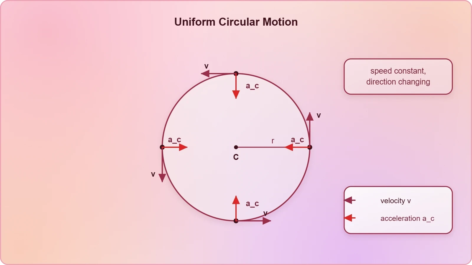
Circular motion at constant speed is the great counterexample to the intuition that acceleration requires a change in speed. An object tracing a circle at steady pace is continuously accelerating because its velocity vector keeps turning. That acceleration points toward the centre, perpendicular to the instantaneous velocity, and its magnitude is ##a_c = \dfrac{v^2}{r}##.

The force responsible for this inward acceleration is called centripetal, meaning centre-seeking. It is not a new kind of force but a role played by tension, gravity, friction, or normal reaction depending on context. A satellite in orbit experiences gravity as its centripetal force; a car turning a corner relies on tyre friction.

Period, Frequency, and Angular Speed

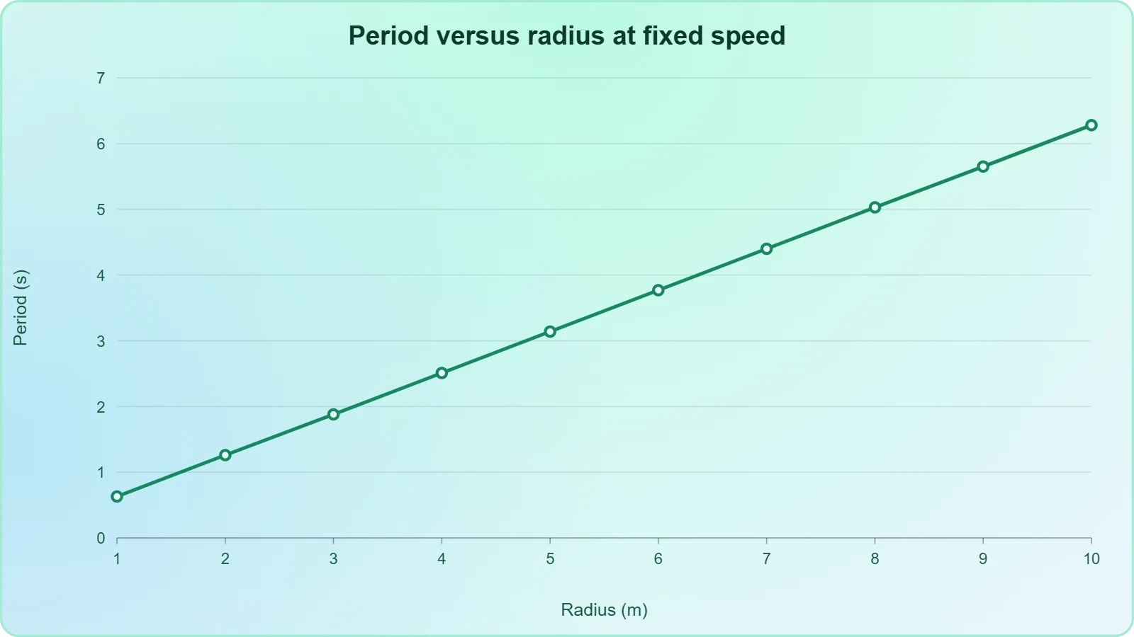
Uniform circular motion is conveniently described by angular quantities. Angular speed ##\omega = \dfrac{v}{r}## measures radians swept per second, and the period ##T = \dfrac{2\pi r}{v}## gives the time for one complete revolution. Frequency is simply the reciprocal of the period, expressed in hertz.

These relationships connect linear and rotational descriptions of the same motion, a bridge that becomes essential when you later study rotational dynamics. For now, note that doubling the radius while holding speed constant halves the angular speed and doubles the period, a proportionality worth internalising.

Where Projectile and Circular Ideas Meet

The two topics converge in problems involving objects launched from rotating platforms or satellites transitioning between orbits. In each case, you resolve velocities into components, apply gravity as the sole external influence, and track how the velocity direction evolves. The mathematics is continuous even when the textbook chapters are not.

A ball released from a spinning merry-go-round, for instance, leaves tangentially with the instantaneous velocity it possessed at release. From that moment it is a projectile, and its subsequent path is a parabola. Recognising the handover point between circular and projectile phases is precisely the integrative skill this lesson cultivates.

Relative Motion Revisited Through a Component Lens

The previous lesson established that velocities transform between frames according to ##\vec{v}_{AB} = \vec{v}_{A} - \vec{v}_{B}##. What deserves emphasis now is how naturally this subtraction fits the component framework. Resolve both velocities into ##x## and ##y## parts, subtract like with like, then recombine. The river-crossing problem becomes almost mechanical.

This method scales gracefully. Whether you are computing the drift of an aircraft in crosswind or the apparent motion of rain seen from a moving car, the procedure is identical: identify the two frames, express velocities as vectors, subtract, and interpret the result. No new physics is required, only disciplined bookkeeping.

Choosing Axes Wisely

Axis selection is a strategic decision, not a fixed rule. Aligning one axis with the direction of relative motion often collapses a two-dimensional problem into a single equation. Conversely, aligning axes with the ground simplifies problems where gravity dominates. Skilled solvers choose axes to minimise algebra before writing anything down.

Rotating the coordinate system does not change physical reality, only its description. This invariance is a quiet but powerful principle, and it foreshadows the coordinate transformations you will meet in more advanced mechanics. For now, practise switching axes deliberately and comparing the resulting equations.

Diagnostic Check: Spotting the Right Model

Many learners struggle not with algebra but with classification. Is this a projectile, a circular-motion problem, or a relative-velocity puzzle? A short diagnostic routine resolves the ambiguity quickly, and the table below summarises the decision cues that experienced problem-solvers apply almost unconsciously.

Ask first whether gravity is the only force after launch. If yes, treat it as a projectile. If a constraint forces circular travel, invoke centripetal analysis. If two observers disagree about velocity, reach for relative subtraction. These three questions cover the overwhelming majority of planar kinematics exercises.

Computational Verification of Trajectories and Orbits

Analytical formulas are elegant, but numerical simulation offers a complementary form of understanding. By stepping through time in small increments and updating velocity and position, you can watch a projectile arc or a circular orbit emerge from the same few lines of code. This exercise also reveals where idealised formulas break down.

The snippet below integrates projectile motion using a simple Euler scheme. It is deliberately minimal, yet it reproduces the parabolic path and lets you experiment with launch angles and drag terms. Running it alongside the closed-form range equation builds genuine confidence in both approaches.

import math

def projectile(u, theta_deg, g=9.8, dt=0.01):
    theta = math.radians(theta_deg)
    vx, vy = u * math.cos(theta), u * math.sin(theta)
    x, y = 0.0, 0.0
    path = [(x, y)]
    while y >= 0:
        vx, vy = vx, vy - g * dt
        x, y = x + vx * dt, y + vy * dt
        path.append((x, y))
    return path

trajectory = projectile(30, 45)
print("Range:", round(trajectory[-1][0], 2), "m")

Reading the Output Critically

The printed range should land near the analytical value of roughly 91.8 metres, with small discrepancies arising from the finite time step. Reducing ##dt## tightens the agreement, illustrating a general principle: numerical error shrinks as resolution improves, but never vanishes entirely. This awareness prepares you for the graphical analysis lesson ahead.

Extend the same loop to include a drag term proportional to velocity squared, and the trajectory becomes asymmetric, with a steeper descent than ascent. Real projectiles behave this way, which is why idealised range formulas overestimate actual distances. The simulation makes that gap tangible rather than abstract.

From Simulation to Insight

Simulation is not a substitute for theory but a dialogue partner. When the code and the formula disagree, either the discretisation is too coarse or a physical assumption has been violated. Diagnosing which is which sharpens both programming judgement and physical intuition, a pairing increasingly valued in modern physics education.

Try varying the launch angle across the table values and confirm the symmetry between complementary angles. Then introduce drag and watch the symmetry dissolve. These small experiments transform passive formulas into active understanding, which is precisely the integrative aim of this lesson.

Consolidating the Framework Before Graphical Analysis

Integration is the theme that binds this lesson together. Vectors supply the language, projectiles and circular motion supply the two canonical applications, and relative velocity supplies the frame-shifting tool. Seen together, they form a single analytical system rather than three disconnected chapters, and that unity is what you should carry forward.

The next lesson turns to graphical analysis, where velocity-time and displacement-time curves reveal motion qualitatively before any equation is written. Everything practised here, especially component reasoning and the independence of perpendicular motions, will make those graphs readable at a glance. The groundwork is deliberately laid.

A Short Self-Assessment Routine

Before moving on, test yourself with three questions. Can you derive the range formula from component equations without consulting notes? Can you explain why centripetal acceleration exists despite constant speed? Can you subtract two velocity vectors in component form and interpret the result physically? Affirmative answers indicate readiness.

Where any answer falters, revisit the corresponding section rather than pressing ahead. Spaced revisiting of these core derivations pays compound interest later, particularly when rotational dynamics and orbital mechanics arrive. The habit of self-testing is itself a transferable skill worth cultivating deliberately.

Looking Ahead to Graphs and Beyond

Graphical analysis will ask you to extract acceleration from the slope of a velocity-time curve and displacement from the area beneath it. Those operations are simply the calculus of the equations you have used, presented visually. Familiarity with the formulas makes the graphs meaningful rather than mysterious.

Beyond this course, the same framework extends to electric fields, fluid flow, and orbital mechanics, all of which treat motion in two or three dimensions with vector tools. What feels like a self-contained topic is actually a gateway, and the integrative perspective developed here will serve you repeatedly.