Relative Velocity in Two Dimensions

Relative velocity is the conceptual hinge on which two-dimensional kinematics turns from abstract vector algebra into practical reasoning about the physical world. When a boat crosses a river, a pilot corrects for crosswind, or a passenger watches rain streak sideways through a moving train window, each observer measures a different velocity for the same event. Lesson 16 of this thirty-part course isolates that idea and gives it rigorous mathematical form, building directly on the centripetal force discussion that preceded it while preparing the ground for the integrative synthesis that follows.

What distinguishes this treatment is its insistence that velocity is never absolute but always referenced to a chosen frame. Learners encounter the subtraction rule for relative velocity, learn to decompose motion into independent components, and apply the resulting expressions to river-crossing, aircraft-drift, and pursuit scenarios. Each worked example is designed to convert a formula into a mental picture, so that the mathematics of moving observers becomes intuitive rather than mechanical.

Because relative motion underpins everything from radar tracking to orbital rendezvous, the lesson also connects classroom vectors to genuine engineering practice. By the close, readers should be able to translate any two-observer problem into a clean vector diagram, resolve it algebraically, and interpret the answer physically. That competence is precisely what the next lesson, which consolidates motion in a plane, will assume as given.

Frames of Reference and the Meaning of Relative Motion

Every velocity measurement presupposes a coordinate frame, an implicit or explicit grid against which positions are recorded and timed. Galileo first articulated this insight when he noted that a passenger below decks on a smoothly moving ship cannot distinguish rest from uniform motion by any mechanical experiment. The principle remains foundational: physics does not privilege one inertial frame over another, and relative velocity is the bookkeeping that translates between them.

Why Absolute Velocity Is Unobservable

No experiment performed entirely within a closed, uniformly moving laboratory can reveal that laboratory's velocity through space. This is the Galilean relativity principle, and it explains why the phrase "the train travels at 120 km/h" is shorthand for "the train travels at 120 km/h relative to the ground." Without a stated reference, a velocity figure is incomplete rather than merely imprecise.

The practical consequence is liberating. We may attach a frame to the ground, to a moving car, or to a drifting balloon, whichever simplifies the algebra. Answers computed in different frames must agree once transformed, and that consistency requirement becomes a powerful check on any solution. Choosing the frame wisely is therefore the first strategic decision in every relative-motion problem.

Inertial Frames and the Galilean Transformation

An inertial frame moves at constant velocity without rotation, so Newton's laws hold within it unchanged. If frame ##S'## moves with constant velocity ##\vec{u}## relative to frame ##S##, positions transform according to ##\vec{r}' = \vec{r} - \vec{u}t##, and differentiating once yields the velocity relation that governs all that follows. Acceleration, differentiated twice, is identical in both frames.

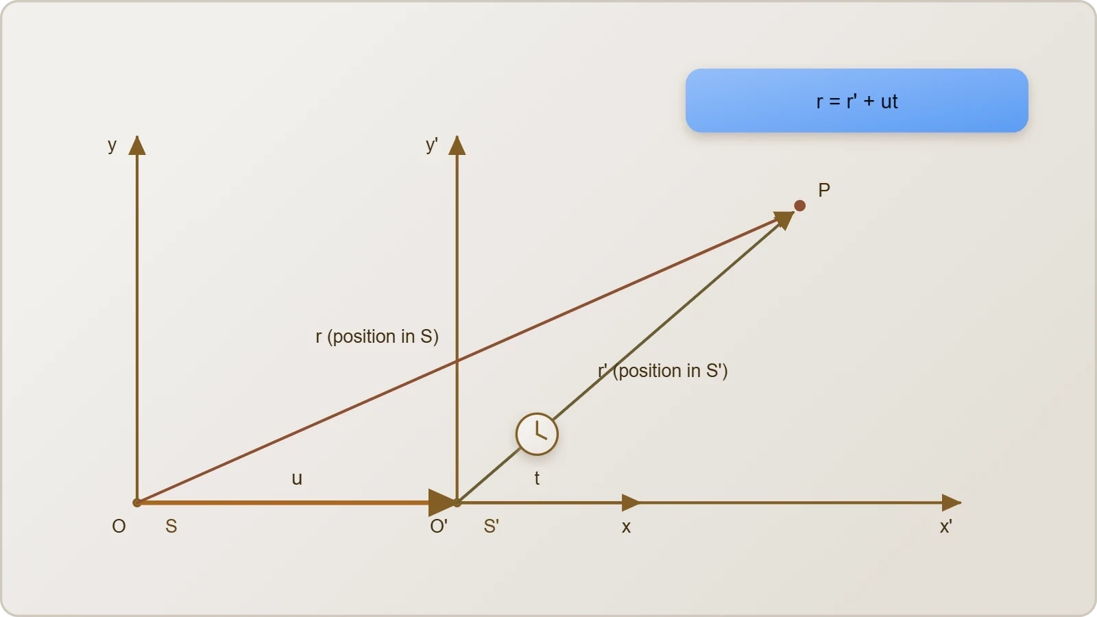
That final equality carries real weight: because ##\vec{a}' = \vec{a}##, forces and masses need no correction when switching between inertial frames. Only velocities shift, and they shift by simple vector subtraction. This asymmetry between velocity and acceleration is the mathematical heart of Galilean relativity and the reason relative-velocity problems reduce to geometry rather than dynamics.

The Relative Velocity Equation and Its Vector Geometry

With frames defined, the central relation can be stated compactly and then unpacked geometrically. The velocity of object A as measured by observer B equals the velocity of A relative to the ground minus the velocity of B relative to the ground. Written as a vector equation, it is deceptively simple, yet nearly every two-dimensional relative-motion problem is an exercise in applying it correctly.

Deriving the Subtraction Rule

Let ##\vec{v}_{A}## and ##\vec{v}_{B}## denote the velocities of A and B in the ground frame. In time ##t##, their displacements are ##\vec{v}_{A}t## and ##\vec{v}_{B}t##, so the displacement of A as seen by B is their difference. Dividing by ##t## gives the relative velocity directly.

The notation rewards care: ##\vec{v}_{AB}## reads "velocity of A relative to B," and reversing the subscripts negates the vector, so ##\vec{v}_{BA} = -\vec{v}_{AB}##. This antisymmetry is a useful consistency check. If two cars approach each other head-on at equal speeds ##v##, each measures the other closing at ##2v##, not ##v##, because the subtraction aligns the vectors.

Solving with Components and Diagrams

In two dimensions the subtraction is performed component-wise, which converts a vector problem into two independent scalar problems. Resolving along perpendicular axes and applying the rule to each component separately keeps signs straight and prevents the classic error of subtracting magnitudes while ignoring direction.

import numpy as np

def relative_velocity(v_a, v_b):
    """Velocity of A as measured in the frame of B."""
    return np.subtract(v_a, v_b)

def speed_and_heading(vec):
    speed = np.linalg.norm(vec)
    heading = np.degrees(np.arctan2(vec[1], vec[0]))
    return speed, heading

car_a = np.array([25.0, 0.0])   # m/s, eastbound
car_b = np.array([-15.0, 0.0])  # m/s, westbound

v_ab = relative_velocity(car_a, car_b)
print(speed_and_heading(v_ab))  # closing speed 40 m/s, heading 0 deg

A scale diagram drawn before any algebra remains the most reliable safeguard. Sketch both ground-frame vectors tail to tail, then draw the vector from the tip of ##\vec{v}_{B}## to the tip of ##\vec{v}_{A}##; that arrow is ##\vec{v}_{AB}##. Learners who habitually draw this triangle rarely misapply the formula under examination pressure.

River-Crossing Problems: Steering, Drift, and Minimum Time

River problems are the canonical testing ground for relative velocity because they combine a moving medium with a moving body and a fixed bank. A swimmer or boat has a velocity relative to the water, the water itself drifts relative to the bank, and the ground-frame velocity is the vector sum. Two natural questions follow: how to cross in the shortest time, and how to land directly opposite the starting point.

Shortest-Time Crossing

Crossing time depends only on the component of velocity perpendicular to the banks, since the river's width is fixed. Pointing the boat straight across maximizes that component, giving ##t_{min} = d/v_{b}##, where ##d## is the width and ##v_{b}## the boat's speed relative to water. The current then sweeps the boat downstream by ##v_{r}t_{min}##, a drift that cannot be avoided if time is the priority.

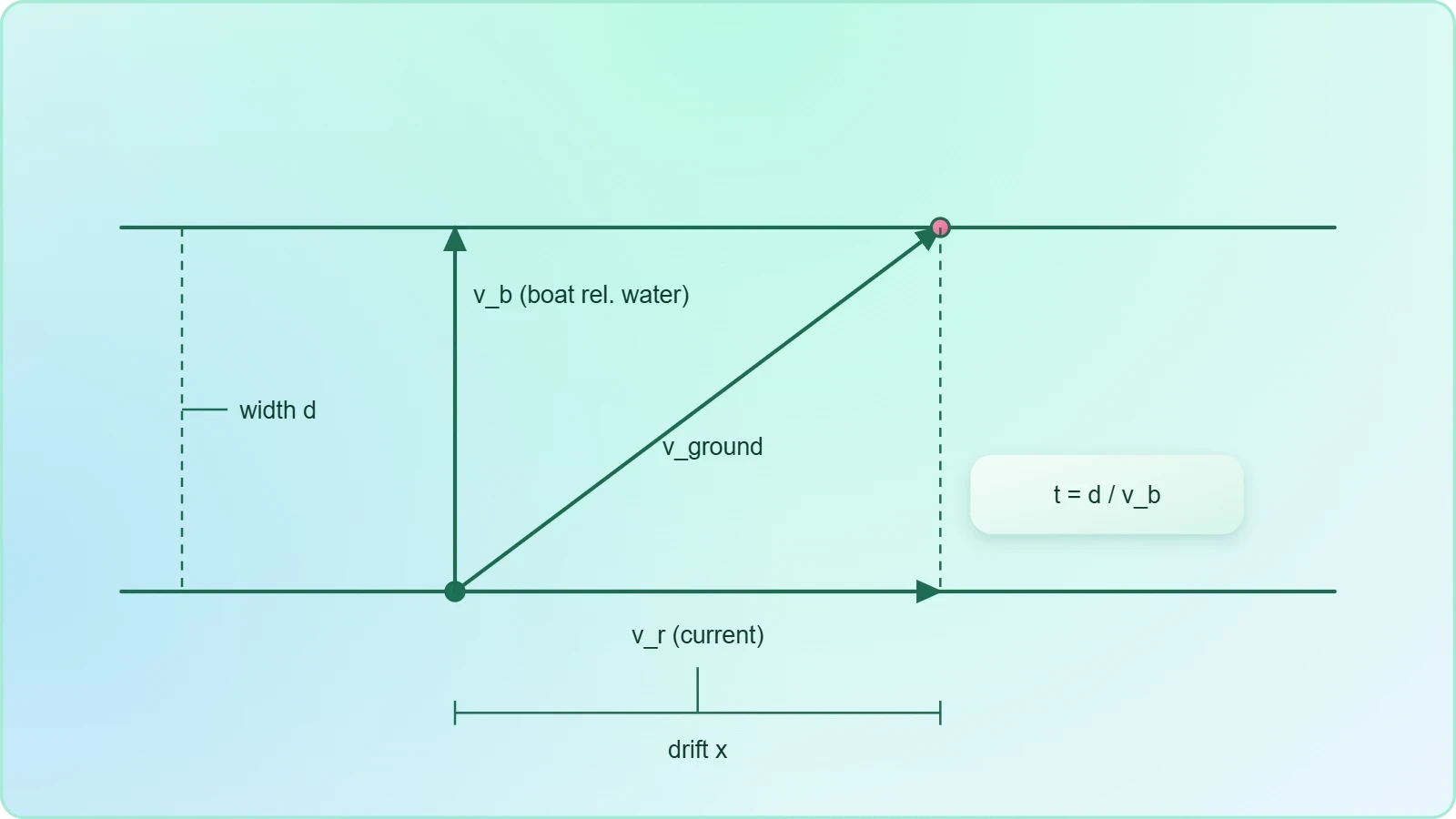
This result surprises many beginners, who assume aiming upstream shortens the trip. It does not: any upstream tilt reduces the perpendicular component and lengthens the crossing. The lesson generalizes neatly, because the same decomposition logic governs aircraft drift and any transport problem involving a moving medium.

Zero-Drift Crossing and the Drift Formula

To land directly opposite, the boat must be angled upstream so that its upstream component exactly cancels the current. The required heading satisfies ##\sin\theta = v_{r}/v_{b}##, which has a solution only when the boat is faster than the river. The resulting crossing time is longer than the minimum, since the effective perpendicular speed is reduced.

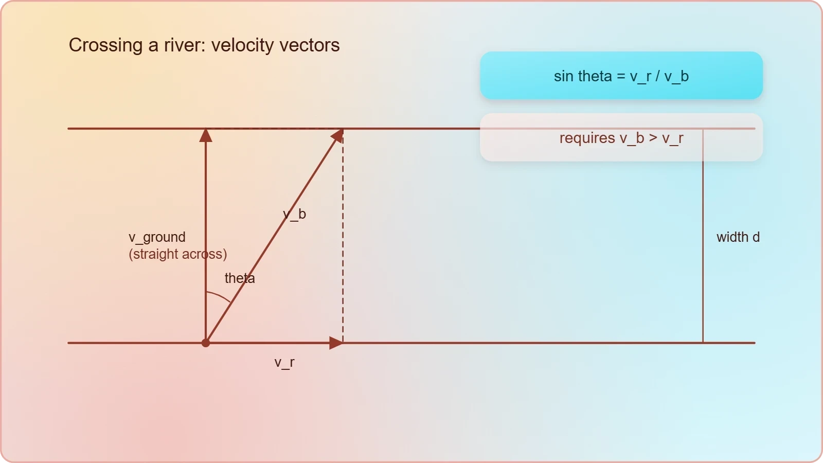
When the current exceeds the boat's speed, no heading achieves zero drift, and the best strategy is to minimize drift by pointing upstream as far as possible. The drift for a straight-across heading, ##x = v_{r}d/v_{b}##, quantifies the penalty. These formulas appear repeatedly in entrance examinations, so deriving them once from first principles pays lasting dividends.

Rain, Wind, and Moving Observers in Everyday Settings

Relative velocity explains a family of familiar phenomena that otherwise seem paradoxical. Rain that falls vertically appears slanted to a driver, wind that is calm on the ground buffets a cyclist, and a thrown ball curves oddly when viewed from a moving cart. Each case is the same subtraction rule applied to a different pair of observers, and each yields to the same diagrammatic method.

The Slanting Rain Problem

Rain falling vertically at speed ##v_{r}## appears to a driver moving horizontally at ##v_{c}## to come from ahead and above. The rain's velocity relative to the car is ##\vec{v}_{r} - \vec{v}_{c}##, a vector tilted from the vertical by an angle satisfying ##\tan\theta = v_{c}/v_{r}##. Faster driving therefore produces a more horizontal apparent rainfall.

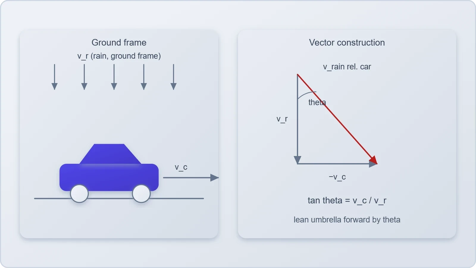
The practical corollary concerns umbrellas and windscreens: the tilt angle tells you exactly how much to lean the canopy forward. This is a satisfying instance where a vector subtraction predicts a quotidian experience, and it reinforces the habit of asking "relative to what?" before accepting any velocity statement.

Wind Triangle for Aircraft Navigation

Aircraft navigation formalizes the same geometry. The heading and airspeed define the plane's velocity relative to the air, the wind defines the air's velocity relative to the ground, and their vector sum is the ground track. Pilots solve the wind triangle to determine the heading that produces a desired course over the ground.

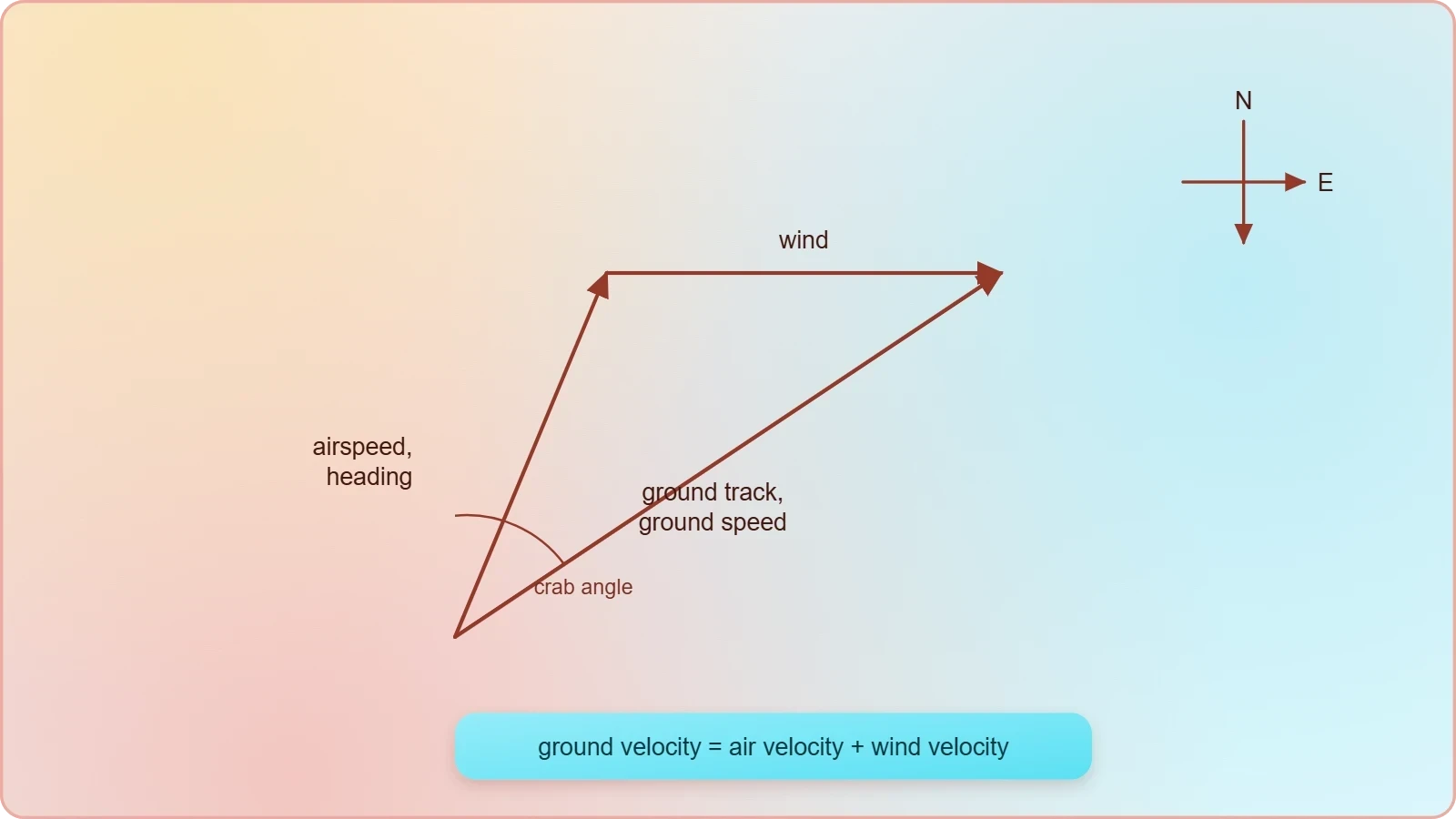
Crosswind components demand a crab angle, while headwinds and tailwinds alter ground speed without changing airspeed. Because fuel consumption tracks airspeed while arrival time tracks ground speed, the distinction has operational consequences. The mathematics is identical to the river problem, merely rotated into the sky and dressed in aviation vocabulary.

Pursuit, Interception, and Closest Approach

Beyond crossing problems lies a richer class in which one moving object chases or intercepts another. A patrol boat pursuing a smuggler, a missile tracking a target, or two ships on converging courses all reduce to relative velocity once the frame is shifted to one of the objects. In that frame the pursuer's motion becomes a straight line, and questions of interception or minimum separation become elementary geometry.

Interception Conditions

Interception requires that the relative velocity vector point along the line joining the two objects at the moment of decision. If the pursuer is faster, a unique heading satisfies this condition; if slower, interception may be impossible depending on geometry. Solving for the required heading is a standard application of the sine rule to the velocity triangle.

The time to interception follows from dividing the initial separation by the component of relative velocity along the line of sight. This single formula covers pursuit curves, torpedo problems, and rendezvous planning, and it demonstrates how a change of frame can dissolve apparent complexity into a one-line calculation.

Minimum Separation and Closest Approach

When interception is not required, the natural question is how close two objects come. In the frame of one object, the other travels along a straight line, and the minimum separation is simply the perpendicular distance from the observer to that line. No calculus is needed, only the projection of the initial position onto the relative velocity direction.

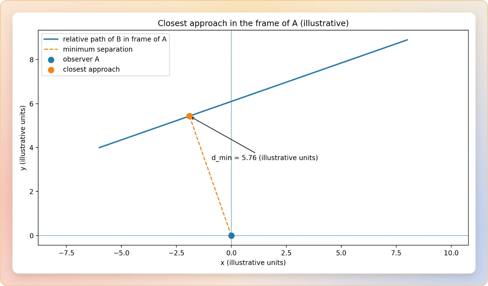
This cross-product expression is compact and dimensionally sound, and it generalizes to three dimensions without modification. Air-traffic conflict detection and maritime collision-avoidance systems rely on precisely this computation, which is why the closest-approach concept deserves attention beyond the classroom.

Worked Examples and Common Pitfalls

Mastery of relative velocity comes from disciplined practice rather than formula memorization. The examples below progress from a straightforward one-dimensional check to a full two-dimensional interception, illustrating the method at each stage. Alongside them, the recurring errors that cost marks in examinations are identified and corrected, so that learners can audit their own work before submitting it.

Step-by-Step Worked Problems

Consider a boat with water speed 4 m/s crossing a 300 m river flowing at 3 m/s. Aiming straight across, the crossing takes 75 s and the drift is 225 m. To land opposite, the heading must satisfy ##\sin\theta = 3/4##, giving about 48.6 degrees upstream and a crossing time near 113 s.

Now consider two ships, one steaming east at 20 km/h and another north at 15 km/h, initially 50 km apart on perpendicular courses. In the first ship's frame the second moves along a straight line, and the closest approach is found by projecting the initial separation onto that relative velocity. The arithmetic is short once the frame is chosen.

Diagnosing Frequent Errors

The most common mistake is subtracting speeds as scalars when the vectors are not collinear, which silently discards direction. A second frequent error is confusing the observer's frame with the ground frame midway through a calculation, producing sign inconsistencies. A third is forgetting that crossing time depends only on the perpendicular component.

Careful notation prevents all three. Label every velocity with both subscripts, draw the vector triangle before substituting numbers, and check that the answer's direction makes physical sense. These habits, more than any formula, distinguish reliable problem-solvers from those who merely recognize patterns.

Consolidation and the Bridge to Plane Motion Synthesis

Lesson 16 closes the conceptual arc that began with vector definitions and passed through projectile trajectories and circular motion. Relative velocity supplies the final ingredient: the recognition that every kinematic description is frame-dependent, and that switching frames is a legitimate and often decisive problem-solving move. With this tool in hand, learners can treat moving observers as ordinary observers once the transformation is applied.

Key Takeaways from This Lesson

The subtraction rule ##\vec{v}_{AB} = \vec{v}_{A} - \vec{v}_{B}## governs all two-dimensional relative motion, and its component form makes computation routine. River crossings, wind triangles, and pursuit problems are variations on one theme, distinguished only by which vectors are known. Closest approach and interception follow from the same frame shift.

Equally important is the conceptual residue: velocity is relational, acceleration is not, and inertial frames are interchangeable. These ideas recur throughout mechanics, from collision analysis to orbital dynamics, and they will reappear whenever the course treats systems with multiple moving parts. The next lesson draws all of plane motion together into a unified synthesis.

Preparing for the Integrative Lesson

The forthcoming synthesis will combine vectors, projectiles, circular motion, and relative velocity into composite problems requiring several tools at once. Learners should arrive fluent in frame selection and vector decomposition, since those skills determine how quickly a complex scenario can be reduced to manageable pieces. Reviewing the worked examples above is the most efficient preparation.

Beyond this course, relative velocity reappears in special relativity, where the Galilean rule is corrected at speeds approaching ##c##, and in fluid mechanics, where moving control volumes demand the same bookkeeping. The beginner who internalizes the subtraction rule now builds a foundation that will support far more advanced study later.