Projectile Motion: Angled Launch

Angled projectile motion represents the point where two-dimensional kinematics becomes genuinely expressive, because the launch angle governs everything that follows: how long the object stays airborne, how high it climbs, and how far it travels before returning to its starting elevation. Where the previous lesson confined the analysis to horizontal launches, this lesson restores the vertical component of initial velocity and examines the consequences systematically. The mathematics remains the same superposition of independent horizontal and vertical motions, but the initial conditions now carry a direction, and that single change produces a rich family of trajectories.

Understanding angled launches matters far beyond textbook exercises. Artillery calculations, sports biomechanics, fountain design, fireworks safety envelopes, and even the ballistic trajectories of volcanic ejecta all rest on the relationships derived here. Engineers routinely invert these equations, working backwards from a required range or clearance height to determine the necessary launch speed and angle. Mastering the forward problem, predicting the trajectory from given initial conditions, is therefore the essential prerequisite for the inverse design problems that follow in the next lesson.

This lesson builds directly on the horizontal-launch foundation, treating the angled case as a natural generalisation rather than a new phenomenon. You will derive the time of flight, maximum height, and horizontal range from first principles, examine the symmetry properties of the parabolic path, and discover why complementary angles share a common range. Each result is connected to its physical interpretation, so the formulas become memorable consequences of reasoning rather than items to memorise.

Decomposing an Angled Launch into Components

An angled launch is defined by two initial parameters: the launch speed ##v_0## and the angle ##\theta## measured above the horizontal. These two numbers encode the entire initial state of the projectile, and every subsequent quantity in this lesson flows from them. The first analytical step is always the same: resolve the initial velocity into horizontal and vertical components using trigonometry.

Resolving the Initial Velocity Vector

The horizontal component is ##v_{0x} = v_0\cos\theta## and the vertical component is ##v_{0y} = v_0\sin\theta##. These projections follow directly from the right-triangle geometry of the velocity vector, with the angle placed between the vector and the horizontal axis. Notice that the two components trade magnitude as the angle varies, which is the origin of nearly every result in this lesson.

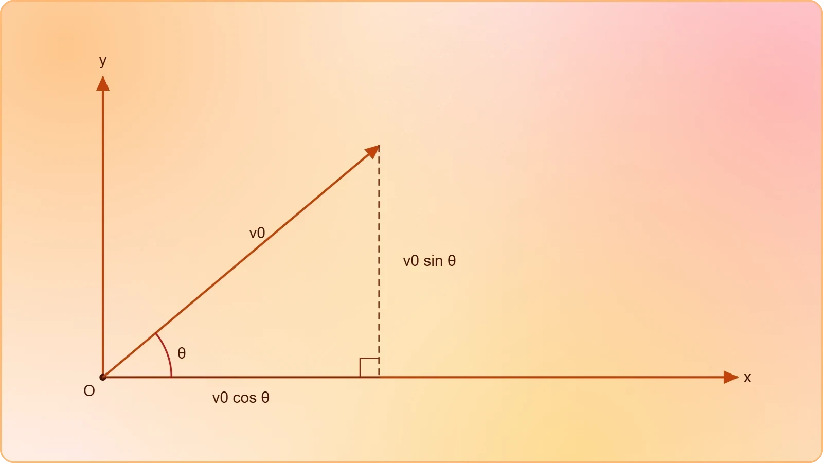
Once resolved, the two components evolve independently. The horizontal component remains constant throughout the flight because no horizontal force acts on the projectile, neglecting air resistance. The vertical component, by contrast, changes uniformly under gravity at a rate of ##g## downward, exactly as in one-dimensional free fall. This separation of concerns is the analytical engine of the entire method.

Setting Up the Equations of Motion

With the origin at the launch point and upward taken as positive, the position equations become ##x(t) = v_0\cos\theta\, t## and ##y(t) = v_0\sin\theta\, t - \tfrac{1}{2}gt^2##. The velocity equations are ##v_x(t) = v_0\cos\theta## and ##v_y(t) = v_0\sin\theta - gt##. Together these four expressions fully determine the motion at any instant.

The trajectory itself is obtained by eliminating time between the position equations, yielding the parabolic path equation below. This single relation describes the shape of the flight and will be used repeatedly when analysing range, clearance, and impact conditions in later sections.

Time of Flight and the Symmetry of the Parabola

The time of flight is governed entirely by the vertical motion, because the projectile returns to its launch elevation when the vertical displacement returns to zero. Setting ##y(t) = 0## in the vertical position equation and factoring out the time yields two solutions: the launch instant itself and the landing instant. The non-trivial solution gives the total airborne duration.

Deriving the Time of Flight

Solving ##v_0\sin\theta\, t - \tfrac{1}{2}gt^2 = 0## produces the time of flight below. The result is elegantly simple: the duration depends only on the vertical component of launch velocity and the gravitational acceleration, with no reference to the horizontal motion whatsoever.

This expression also reveals the ascent time. The projectile reaches its peak when the vertical velocity vanishes, which occurs at ##t = v_0\sin\theta / g##, exactly half the total flight time. The descent therefore mirrors the ascent in duration, a direct consequence of the constant downward acceleration acting symmetrically about the apex.

Symmetry Properties of the Trajectory

For a projectile landing at its launch height, the path is symmetric about the apex in several respects. The speed at any given height on the way down equals the speed at the same height on the way up, and the vertical velocity simply reverses sign. The horizontal velocity, of course, never changes at all.

This symmetry is a powerful problem-solving shortcut. Questions about the speed at a particular height, or the time spent above a certain elevation, can often be answered by reasoning about the mirrored halves of the flight rather than by solving quadratics. Recognising symmetry converts algebra into insight.

Maximum Height and the Apex Condition

The maximum height of an angled projectile is reached at the apex, where the vertical velocity component momentarily becomes zero before reversing. This condition, ##v_y = 0##, is the key that unlocks the height calculation. Substituting the ascent time into the vertical position equation then delivers the peak elevation directly.

Deriving the Maximum Height

Evaluating the vertical position at ##t = v_0\sin\theta/g## gives the maximum height formula shown below. The height scales with the square of the vertical velocity component, so doubling the launch speed quadruples the peak height, a scaling that surprises many beginners.

An equivalent derivation uses the time-free kinematic relation ##v_y^2 = v_{0y}^2 - 2gy##, setting the final vertical velocity to zero. Both routes agree, and comparing them is a useful exercise in choosing the most economical equation for a given problem. The time-free relation is often faster when time is neither given nor requested.

Interpreting the Height Dependence

Because the sine function peaks at 90 degrees, a vertical launch maximises height, while a horizontal launch produces none at all. The height formula therefore interpolates smoothly between the two extremes examined in adjacent lessons. For a fixed speed, steep launches trade range for altitude in a predictable, quantifiable way.

Practical applications exploit this trade-off constantly. Firefighters aiming water jets at upper-storey windows choose steep angles to gain height, accepting a shorter horizontal reach. Conversely, athletes seeking distance flatten their launch angle, sacrificing altitude for range. The same equation governs both decisions.

Horizontal Range and the Complementary Angle Rule

The horizontal range is the total distance travelled along the ground before the projectile returns to its launch elevation. Because the horizontal velocity is constant, the range is simply the horizontal component multiplied by the total time of flight. Combining the two earlier results produces one of the most celebrated formulas in elementary mechanics.

Deriving the Range Equation

Multiplying ##v_0\cos\theta## by the flight time ##2v_0\sin\theta/g## and applying the double-angle identity ##2\sin\theta\cos\theta = \sin 2\theta## yields the range formula below. The compactness of this result conceals a remarkable symmetry that the next subsection explores.

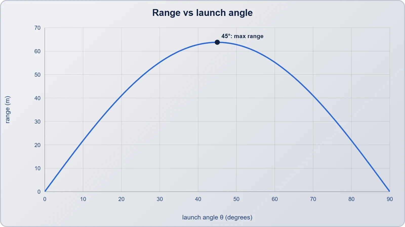
The range depends on the launch angle only through ##\sin 2\theta##, which attains its maximum value of one when ##2\theta = 90°##, that is, when ##\theta = 45°##. For a level landing surface, therefore, a 45-degree launch maximises the horizontal distance for any given speed. This is the familiar optimum taught in every introductory course.

Why Complementary Angles Share a Range

The double-angle form immediately explains a striking fact: angles that sum to 90 degrees produce identical ranges. Since ##\sin 2\theta = \sin(180° - 2\theta)##, a launch at ##\theta## and one at ##90° - \theta## give the same horizontal distance. A 30-degree throw and a 60-degree throw land at the same spot.

The two trajectories are far from identical, however. The steeper launch stays airborne longer and climbs higher, arriving more slowly and descending more vertically. The shallower launch arrives faster and flatter. Range alone does not determine the path, which is why real applications must consider the full trajectory, not just the landing point.

Trajectory Shape and the Envelope of Reach

The parabolic trajectory equation derived earlier describes the path of a single launch completely. But a deeper question arises when the launch speed is fixed and the angle is free to vary: what region of space can the projectile possibly reach? The answer is a bounding parabola, known as the envelope of trajectories, which separates attainable points from unreachable ones.

Reading the Parabolic Path Equation

The trajectory equation ##y = x\tan\theta - gx^2/(2v_0^2\cos^2\theta)## contains the angle in two places, through the slope term and the curvature term. For a given launch, the path is a downward-opening parabola passing through the origin. Its steepness at the origin equals ##\tan\theta##, confirming that the launch angle sets the initial direction of the path.

Differentiating the trajectory equation with respect to ##x## and setting the derivative to zero recovers the apex coordinates, providing an independent check on the maximum height and horizontal position of the peak. This consistency across derivations is a hallmark of well-posed kinematics and a useful verification habit.

The Envelope of All Possible Trajectories

Maximising the height ##y## at a fixed horizontal distance ##x## over all launch angles yields the envelope equation below. Points on or beneath this bounding parabola are reachable with the given speed; points above it are forever out of range, regardless of aim.

The envelope is itself a parabola with its vertex at height ##v_0^2/(2g)## directly above the launch point, the height of a vertical launch. Its intercepts on the ground occur at ##x = \pm v_0^2/g##, twice the maximum range on either side. This elegant construction unifies every possible angled launch into a single geometric boundary.

Worked Example and Computational Verification

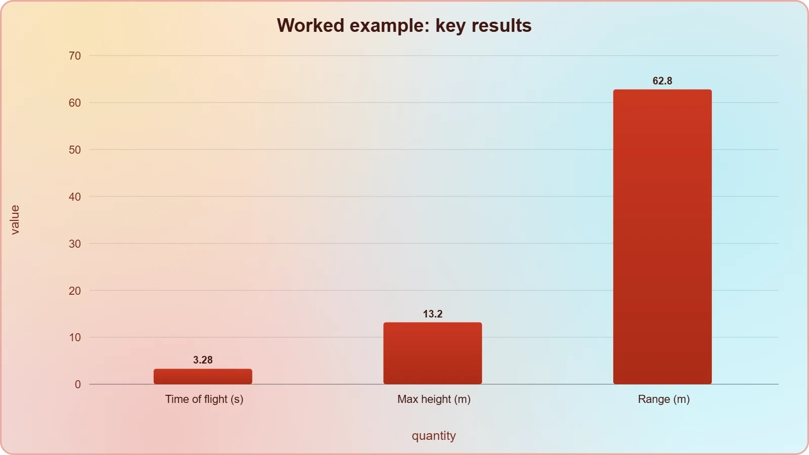
A concrete worked example consolidates the formulas and exposes the order in which quantities should be computed. Consider a ball launched at 25 m/s at 40 degrees above the horizontal from level ground, with air resistance neglected and ##g = 9.8## m/s². The aim is to find the time of flight, maximum height, and range, then verify the results numerically.

Step-by-Step Numerical Solution

The vertical component is ##25\sin 40° \approx 16.07## m/s and the horizontal component is ##25\cos 40° \approx 19.15## m/s. The flight time follows as ##2(16.07)/9.8 \approx 3.28## s. The maximum height is ##(16.07)^2/(2 \times 9.8) \approx 13.2## m, and the range is ##19.15 \times 3.28 \approx 62.8## m.

A useful cross-check applies the range formula directly: ##R = v_0^2\sin 2\theta/g = 625 \times \sin 80°/9.8 \approx 62.8## m, in exact agreement. Such independent verification catches arithmetic slips and reinforces confidence in the derived relations. Students should adopt this double-checking habit routinely.

Simulating the Trajectory in Code

Numerical simulation offers a third route to the same answer and generalises effortlessly to cases with air resistance or uneven terrain. The short script below integrates the equations of motion with a small time step and reports the apex and landing point, which should match the analytical values closely.

import math

v0, theta_deg, g = 25.0, 40.0, 9.8
theta = math.radians(theta_deg)
vx, vy = v0 * math.cos(theta), v0 * math.sin(theta)

dt, t, x, y = 0.001, 0.0, 0.0, 0.0
max_h, flight_time = 0.0, 0.0

while y >= 0.0:
    x += vx * dt
    y += vy * dt
    vy -= g * dt
    t += dt
    max_h = max(max_h, y)
    flight_time = t

print(f"Flight time: {flight_time:.2f} s")
print(f"Max height:  {max_h:.2f} m")
print(f"Range:       {x:.2f} m")

Running the simulation reproduces the analytical results to within the integration error, which shrinks as the time step decreases. The exercise demonstrates that the closed-form formulas and the numerical method describe the same physics, and it prepares the ground for the problem-solving lesson that follows.

Common Pitfalls and the Bridge to Problem Solving

Angled projectile problems are conceptually straightforward but arithmetically unforgiving, and a handful of recurring errors account for most lost marks. The most frequent is mixing up the sine and cosine when resolving components, which silently corrupts every downstream result. A quick sanity check, confirming that the vertical component vanishes at zero angle, catches this immediately.

Frequent Errors and How to Avoid Them

Another common slip is applying the range formula to launches that do not land at the same height as the launch point. The formula ##R = v_0^2\sin 2\theta/g## assumes a level landing, and using it for a cliff launch produces wrong answers. For uneven terrain, return to the vertical position equation and solve for the landing time directly.

Students also forget that the time of flight is not simply twice the ascent time when the landing height differs from the launch height. The symmetry argument holds only for level ground. Recognising the conditions under which each shortcut is valid is as important as remembering the shortcut itself.

Preparing for the Next Lesson

The next lesson shifts from derivation to application, presenting a structured problem-solving methodology for angled launches. The formulas established here become tools rather than destinations, and the emphasis moves to selecting the right equation, managing units, and interpreting results physically. Fluency with the derivations in this lesson is the essential preparation.

Before proceeding, ensure you can reproduce the time of flight, maximum height, and range formulas from first principles without reference. You should also be comfortable explaining why complementary angles share a range and why 45 degrees maximises it. These conceptual anchors will make the problem-solving strategies that follow feel natural rather than mechanical.