Equations of Motion in Two Dimensions

Two-dimensional motion loses none of its predictive power when we stop treating it as a single tangled problem and instead read it as two independent one-dimensional stories unfolding side by side. That is the central insight of this eighth lesson in the course on motion in a plane, and it is the hinge on which everything that follows will turn. Once a learner accepts that horizontal and vertical kinematics can be solved separately and then recombined, the intimidating geometry of curved paths dissolves into familiar algebra.

This lesson deliberately builds on the preceding discussion of acceleration in two dimensions, where the vector nature of changing velocity was established, and it prepares the ground for projectile motion, which arrives next. Rather than repeating vector addition or component resolution, we take those tools as given and apply them to the equations of motion themselves. The result is a compact, reusable toolkit: five kinematic relations, each applied twice, once per axis, with time as the shared thread that stitches the components back together.

Expect a treatment that is rigorous but grounded. We will derive the component equations, examine when the shared-time condition holds and when it quietly fails, and work through numerical examples that mirror real examination and engineering scenarios. By the close, you should be able to take any constant-acceleration problem in a plane and decompose it with confidence, precision, and a clear sense of why the method works.

The Logic of Independent Components

The foundational claim of two-dimensional kinematics is deceptively simple: if acceleration is constant, the motion along any chosen axis is completely unaffected by motion along a perpendicular axis. This independence is not an approximation or a convenient fiction but a direct consequence of vector algebra. Because perpendicular components do not mix under addition, the vector equation of motion splits cleanly into scalar equations that can be solved in isolation.

Consider a particle whose position vector is ##\vec{r} = x\hat{i} + y\hat{j}## and whose constant acceleration is ##\vec{a} = a_x\hat{i} + a_y\hat{j}##. Equating the ##\hat{i}## and ##\hat{j}## coefficients on both sides of the vector kinematic equations yields two separate scalar systems. Each system is identical in form to the one-dimensional equations mastered earlier, which means no new mathematics is required, only disciplined bookkeeping.

Why Perpendicular Axes Do Not Interfere

The physical reason for independence lies in how vectors combine. Adding a horizontal displacement to a vertical displacement produces a diagonal resultant, but the horizontal part of that resultant depends only on the horizontal input. Nothing in the vertical motion can alter the horizontal coordinate, because the two directions are orthogonal and therefore contribute nothing to each other's projections.

This orthogonality is what allows engineers to analyse a bridge cable's tension and a projectile's fall with the same equations. It also explains why a ball dropped from a moving cart lands at the cart's base rather than behind it, a result that surprises students until they recognise that horizontal velocity is preserved independently of the vertical acceleration acting simultaneously.

The Shared-Time Constraint

Although the axes are independent in their equations, they are coupled by a single physical quantity: time. The same interval ##t## appears in both the horizontal and vertical relations, and this shared variable is the bridge that lets us transfer information from one axis to the other. Most two-dimensional problems are solved precisely by exploiting this link.

When a problem supplies a vertical quantity such as fall height, the vertical equation yields ##t##, which is then substituted into the horizontal equation to find range. Conversely, a known horizontal distance can determine flight time, which then fixes the vertical displacement. Recognising which axis offers the easier route to ##t## is the central strategic skill of this lesson.

The Five Equations, Applied Twice

The familiar set of kinematic relations for constant acceleration carries over unchanged, provided each symbol is understood as a component rather than a magnitude. There are five equations linking initial velocity, final velocity, acceleration, displacement, and time. Applied once along ##x## and once along ##y##, they generate ten scalar relations from a single conceptual framework.

What matters pedagogically is not memorising ten formulas but recognising the structure. Each equation omits exactly one variable, so the choice of equation is dictated by which quantity the problem does not mention. This selection logic, already familiar from one-dimensional work, becomes a two-axis decision: first choose the axis, then choose the equation.

Deriving the Component Relations

Starting from the definition of constant acceleration, ##a_x = (v_x - u_x)/t##, rearrangement gives the first component equation. Integrating velocity with respect to time produces the displacement relation, and eliminating time between the two yields the velocity-displacement equation. The vertical axis follows identically, with ##a_y## replacing ##a_x## throughout.

The same three relations hold for the vertical axis with subscript ##y##. Two further equations, expressing displacement in terms of average velocity and in terms of final velocity, complete the set of five. Together they cover every constant-acceleration scenario a beginner will encounter in a plane.

Selecting the Right Equation

Efficient problem-solving begins with an inventory. List the known components, identify the unknown, and note which quantity is absent from the statement. The absent quantity points directly to the appropriate equation, eliminating guesswork and reducing algebraic detours that frequently introduce sign errors.

A useful discipline is to write the inventory as two columns, one per axis, before touching any formula. This habit forces explicit recognition of which quantities belong where, and it exposes immediately whether the problem is underdetermined or whether the shared-time link must be used to close the system.

Sign Conventions and Vector Bookkeeping

Most errors in two-dimensional kinematics are not conceptual but clerical. A misplaced minus sign, an axis direction chosen inconsistently between components, or a velocity resolved with the wrong trigonometric ratio can corrupt an otherwise sound solution. Establishing a sign convention before writing any equation is therefore not pedantry but protection.

The recommended practice is to declare positive directions explicitly, typically rightward for ##x## and upward for ##y##, and to record them at the top of the working. Every component then carries its sign automatically, and the algebra handles direction without further intervention. Consistency across both axes is what preserves the physical meaning of the result.

Resolving Initial Velocity

When a particle is launched at speed ##u## at angle ##\theta## above the horizontal, the initial components follow directly from trigonometry. The horizontal component is ##u\cos\theta## and the vertical is ##u\sin\theta##. These resolved values, not the resultant speed, are what enter the component equations.

A frequent beginner error is to substitute the full launch speed into a vertical equation, which implicitly assumes the entire velocity acts upward. Careful resolution prevents this. The angle must also be measured from a stated reference, since a value quoted relative to the vertical produces swapped sine and cosine terms and a wholly different trajectory.

Recombining Components into Resultants

Once the component solutions are obtained, the physical velocity and displacement are recovered by vector addition. The magnitude of the resultant velocity follows from the Pythagorean relation, and its direction from the inverse tangent of the vertical-to-horizontal ratio. This recombination is the final step, never the first.

Quadrant awareness matters here. The inverse tangent returns a principal value that may require adjustment depending on the signs of the components, particularly when the horizontal velocity is negative. Checking the quadrant against the physical situation guards against reporting a direction that is geometrically plausible but physically wrong.

Worked Example: A Ball Launched at an Angle

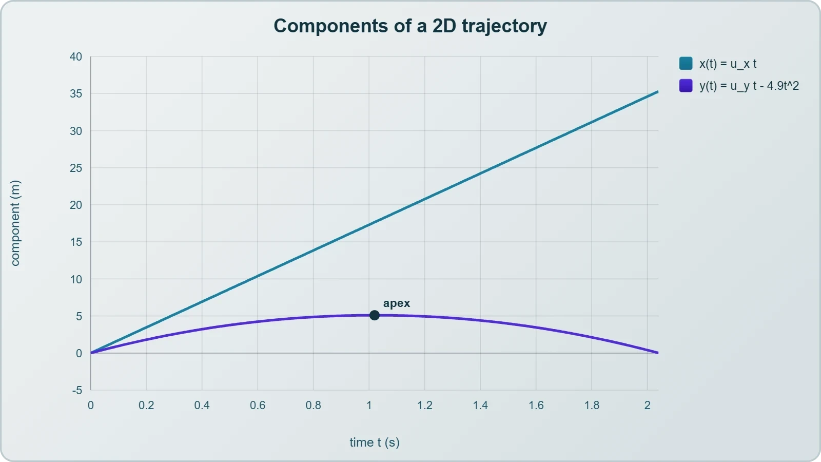
To see the method in action, consider a ball launched from ground level at ##20\,\text{m/s}## at ##30^\circ## above the horizontal, with air resistance neglected and ##g = 9.8\,\text{m/s}^2##. The horizontal component of velocity is approximately ##17.3\,\text{m/s}##, while the vertical component is ##10\,\text{m/s}## upward. These resolved values seed both component systems.

The vertical axis determines the flight time. Setting the vertical displacement to zero at landing and solving the quadratic yields a time of flight near ##2.04\,\text{s}##. Substituting this shared time into the horizontal relation gives a range of roughly ##35.3\,\text{m}##, a result that can be checked against the standard range formula.

Solving the Vertical Axis First

The vertical equation ##y = u_y t - \tfrac{1}{2}gt^2## governs the flight. Setting ##y = 0## produces two roots: the launch instant and the landing instant. The non-zero root is the physically meaningful flight time, and discarding the trivial root is a routine step that beginners sometimes overlook.

Once the flight time is known, the vertical velocity at any instant follows from ##v_y = u_y - gt##. At the apex, where ##v_y = 0##, the time is ##u_y/g \approx 1.02\,\text{s}##, exactly half the total flight time. This symmetry is a useful consistency check on the arithmetic.

Transferring Time to the Horizontal Axis

With the flight time established, the horizontal axis becomes trivial because acceleration there is zero. The range is simply ##u_x t##, and the horizontal velocity remains constant throughout. This asymmetry between the axes, one accelerating and one uniform, is the defining feature of projectile problems to come.

Notice how the solution never required a single equation mixing ##x## and ##y##. The axes were solved in sequence, linked only by the shared time. That is the method in its purest form, and it generalises directly to the projectile motion lesson that follows this one.

Computational Verification of Component Solutions

Modern practice increasingly pairs analytical kinematics with numerical checking, and a short script can confirm every hand calculation in seconds. The value of such verification is not merely catching arithmetic slips but building intuition about how the components evolve together over time. A few lines of code can tabulate position and velocity at each instant.

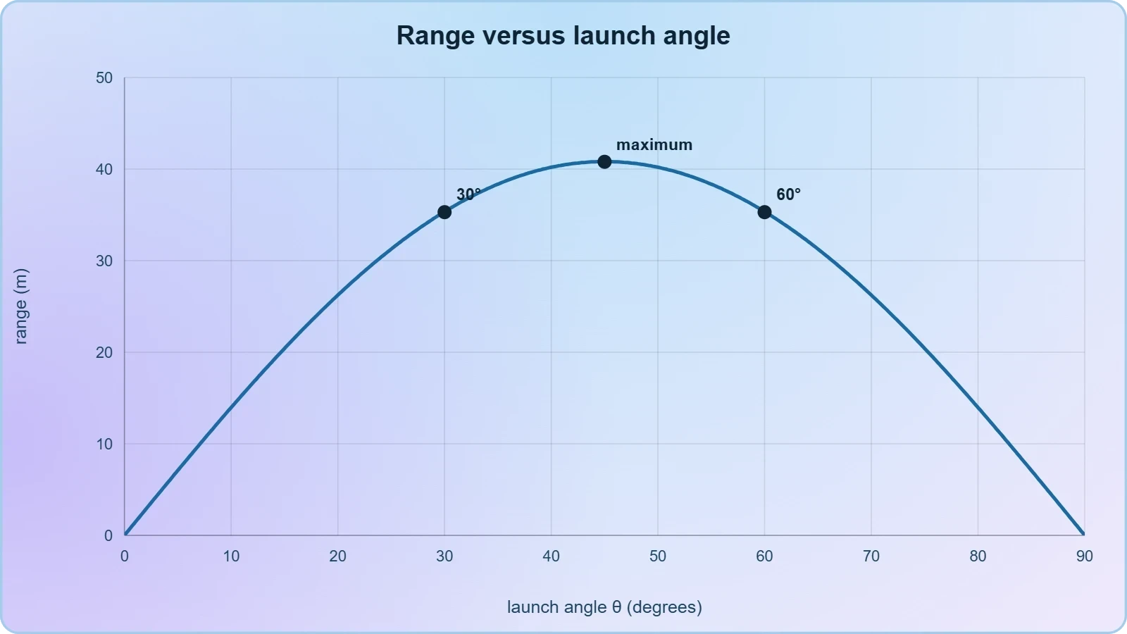
The script below reproduces the worked example, printing the flight time, range, and apex height. Learners are encouraged to modify the launch angle and observe how the range varies, discovering empirically that complementary angles yield equal ranges, a result they will later prove analytically in the projectile lesson.

Python Implementation

The implementation resolves the initial velocity, solves the vertical quadratic for flight time, and then evaluates the horizontal displacement. It deliberately mirrors the manual procedure step by step, so that the correspondence between the algebra and the code remains transparent to a beginner.

import math

u = 20.0          # launch speed in m/s
theta = 30.0      # angle above horizontal in degrees
g = 9.8           # gravitational acceleration

ux = u * math.cos(math.radians(theta))
uy = u * math.sin(math.radians(theta))

# Vertical axis: solve y = uy*t - 0.5*g*t^2 = 0 for the non-zero root
t_flight = 2.0 * uy / g
range_x = ux * t_flight
apex = (uy ** 2) / (2.0 * g)

print(f"Horizontal velocity: {ux:.2f} m/s")
print(f"Vertical velocity:   {uy:.2f} m/s")
print(f"Time of flight:      {t_flight:.2f} s")
print(f"Range:               {range_x:.2f} m")
print(f"Apex height:         {apex:.2f} m")

Interpreting the Output

Running the script returns values matching the hand solution, confirming that the component method and its computational twin agree. More importantly, the output makes the shared-time link visible: the same ##t## value drives both the vertical fall and the horizontal advance, and altering either component changes the trajectory accordingly.

Students who extend the script to sweep angles from zero to ninety degrees will observe the range peaking near ##45^\circ## and falling symmetrically on either side. This exploration prepares the conceptual ground for the next lesson, where projectile motion is treated as a dedicated subject with its own characteristic equations and graphs.

Limits of the Component Method

The component approach rests on one assumption that deserves explicit attention: acceleration must be constant. When acceleration varies with time, position, or velocity, the simple kinematic equations no longer apply, and the problem requires integration or numerical methods. Recognising this boundary prevents the misapplication of formulas beyond their domain.

Air resistance is the most common culprit in practice. It introduces a drag force opposing velocity, making acceleration depend on speed and therefore on time. The resulting motion is no longer parabolic, and the elegant symmetry between ascent and descent disappears. For introductory purposes we neglect drag, but the caveat should be stated rather than hidden.

When Acceleration Varies

If acceleration is a known function of time, the velocity follows by integration, and position by a second integration. The component independence survives this generalisation, since each axis can be integrated separately. What fails is the closed-form algebraic shortcut, not the underlying separability of the axes.

This integral formulation is the natural bridge to calculus-based mechanics, and learners who have met integration will recognise the pattern immediately. Those who have not can still appreciate the qualitative point: variable acceleration demands more than the five standard equations can supply.

Preparing for Projectile Motion

The next lesson narrows the general framework to the special case where horizontal acceleration vanishes and vertical acceleration equals ##-g##. Everything developed here transfers directly, but the symmetry of that case permits additional shortcuts and a richer graphical treatment. The groundwork laid in this lesson ensures those shortcuts are understood rather than merely memorised.

Before moving on, consolidate the method: declare axes, resolve initial velocity, inventory knowns per axis, select equations by the missing quantity, solve each axis, and recombine. This sequence, applied with care, handles every constant-acceleration problem in a plane that a beginner will meet, and it scales gracefully to the projectile problems ahead.