Acceleration in Two Dimensions

Acceleration is the quantity that transforms kinematics from a description of steady motion into a genuine account of how motion evolves. In the previous lesson we established position, displacement, and velocity as vectors, learning that a velocity vector carries both a magnitude and a direction, and that either can change independently. This lesson takes the natural next step: defining acceleration as a vector and examining precisely how it governs changes in velocity across two dimensions. The central insight is deceptively simple yet remarkably powerful — acceleration measures the rate at which velocity changes, and because velocity is a vector, a change in direction alone constitutes acceleration just as surely as a change in speed.

Many learners arrive at this topic carrying a one-dimensional intuition in which acceleration means "speeding up" or "slowing down." That intuition collapses in two dimensions, where a body can move at perfectly constant speed while accelerating continuously. A car rounding a bend, a satellite orbiting Earth, and a ball at the apex of its flight all illustrate this richer behaviour. By the end of this lesson you will be able to compute average and instantaneous acceleration vectors, decompose them into components, interpret their geometric relationship with velocity, and recognise why perpendicular acceleration bends a path without altering speed.

This lesson sits deliberately between the vector groundwork of Lesson 6 and the component equations of motion that follow in Lesson 8. We will not re-derive displacement or velocity; instead we build directly upon them, treating velocity as a known vector function and asking how it changes. The treatment emphasises conceptual clarity and real-world application, supported by worked reasoning, structured data, and a short computational example. Every definition here becomes a working tool in the next lesson, where constant-acceleration equations are applied component by component.

Defining Acceleration as a Vector Quantity

Acceleration is defined as the rate of change of velocity with respect to time, and because velocity is a vector, acceleration inherits vector status automatically. This means acceleration possesses both magnitude and direction, and it must be reported with both to be meaningful. A statement that a body accelerates at ##5\ \text{m/s}^2## is incomplete until we specify the direction of that acceleration relative to the chosen coordinate axes.

Average Acceleration and Its Component Form

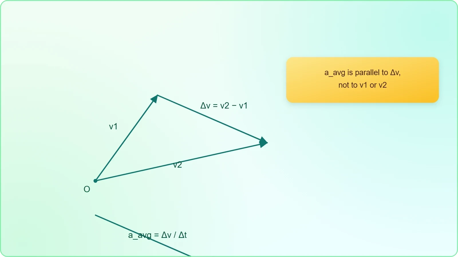
Average acceleration over a time interval is the change in velocity divided by the elapsed time, capturing the net effect of all velocity changes during that window. It tells us the uniform acceleration that would produce the same overall velocity change in the same interval. The definition is written as the difference of two velocity vectors divided by the scalar time interval.

Because vector subtraction is performed component by component, average acceleration resolves neatly into independent horizontal and vertical parts. Each component equals the corresponding velocity change divided by the time interval, so the two-dimensional problem splits into two one-dimensional calculations. This decomposition is the practical bridge to the equations of motion developed in the following lesson.

Instantaneous Acceleration and the Limiting Process

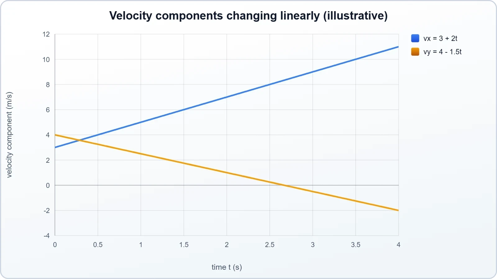
Instantaneous acceleration is obtained by letting the time interval shrink toward zero, turning the average into a derivative of velocity with respect to time. It describes the acceleration at a single instant and can vary continuously along a path. Mathematically it is the time derivative of the velocity vector, evaluated at the moment of interest.

Since velocity is itself the derivative of position, acceleration is the second derivative of the position vector with respect to time. This nesting of derivatives means that a single position function encodes the entire kinematic story. Differentiating once yields velocity; differentiating again yields acceleration, and each step preserves the vector character of the quantity.

Components of Acceleration in Two Dimensions

Resolving acceleration into perpendicular components is the single most useful technique in two-dimensional kinematics. We choose axes, typically horizontal and vertical, and express the acceleration vector as the sum of a component along each axis. Because the axes are independent, the motion along one axis proceeds as though the other axis did not exist, which is the foundation of projectile analysis.

Resolving the Acceleration Vector

Given an acceleration of magnitude ##a## making an angle ##\theta## with the positive x-axis, the components follow directly from trigonometry. The horizontal component is the magnitude multiplied by the cosine of the angle, and the vertical component uses the sine. The magnitude and direction can be recovered from the components using the Pythagorean theorem and the inverse tangent.

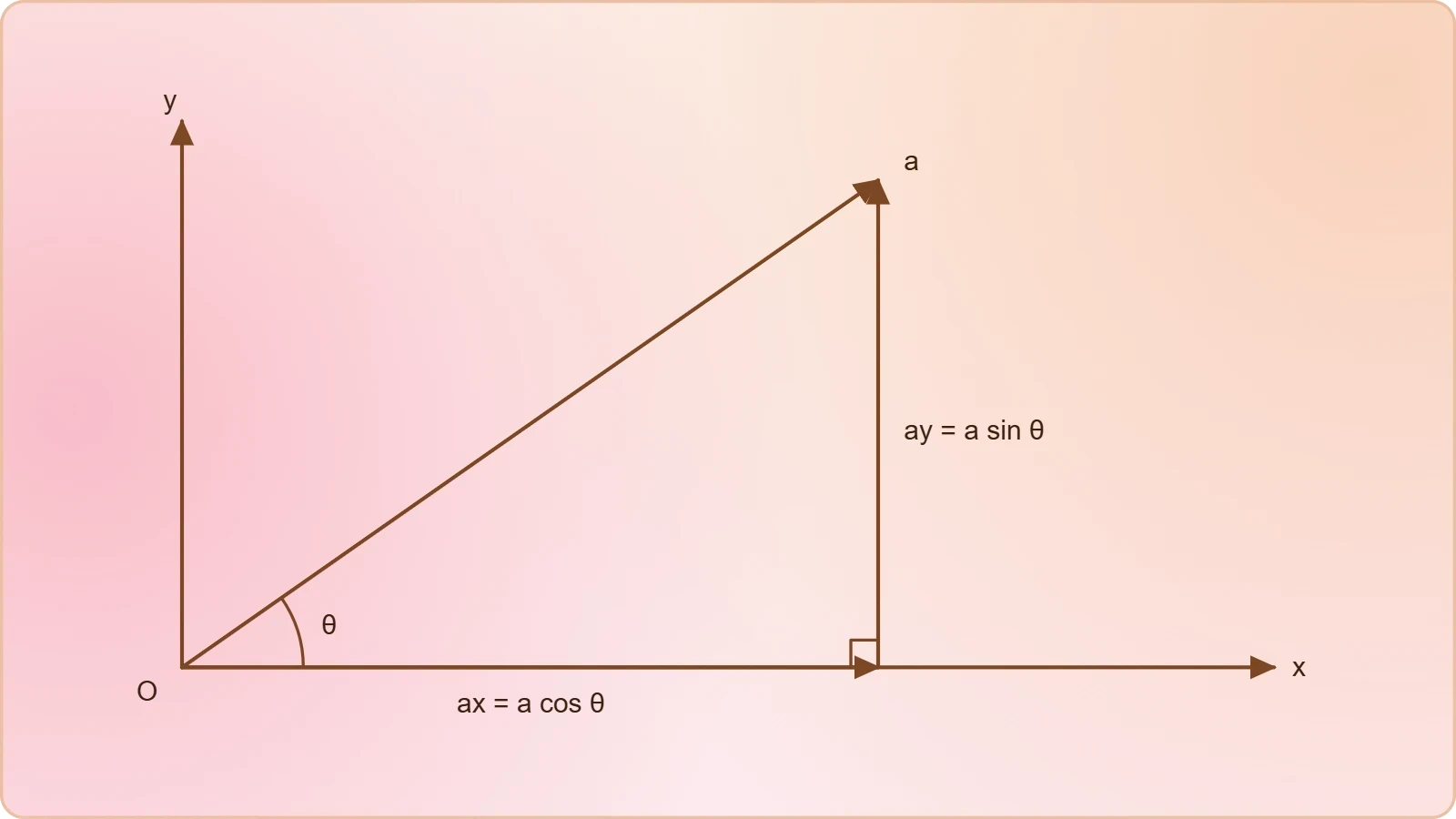
These relations mirror the component treatment of velocity from the previous lesson, and that symmetry is intentional. Every vector operation — addition, subtraction, scaling, and differentiation — is performed component by component. Once you internalise this rule, two-dimensional problems become pairs of familiar one-dimensional problems solved side by side.

Independence of Perpendicular Components

The independence principle states that acceleration along one axis has no effect on motion along the perpendicular axis. A projectile's vertical acceleration due to gravity does not alter its horizontal velocity, which remains constant when air resistance is neglected. This separation is what allows us to predict range and time of flight with such clean equations.

Independence does not mean the components are unrelated in every sense; they share a common time variable. The same clock governs both axes, so the horizontal and vertical motions are synchronised even though their accelerations differ. Recognising this shared time parameter is essential when solving for where and when a projectile lands.

How Acceleration Relates to Velocity Direction

The relationship between acceleration and velocity is geometric, and its interpretation depends entirely on the angle between the two vectors. Acceleration can point in the same direction as velocity, opposite to it, or at any angle in between. Each configuration produces a distinct qualitative behaviour, and mastering this geometry removes much of the confusion surrounding two-dimensional motion.

Parallel and Antiparallel Acceleration

When acceleration is parallel to velocity, the speed increases while the direction of travel remains unchanged. The body simply moves faster along its existing path, and the acceleration acts purely as a tangential influence. This is the familiar case of a car pressing the accelerator on a straight highway.

When acceleration is antiparallel, pointing exactly opposite to velocity, the speed decreases without any change in direction. The body slows along its current line of travel, and if the deceleration persists, the velocity eventually reverses. Braking a bicycle on a straight path is the everyday embodiment of this configuration.

Perpendicular Acceleration and Curved Paths

When acceleration is perpendicular to velocity, the speed remains momentarily constant while the direction of motion changes. The acceleration bends the velocity vector without stretching it, producing a curved trajectory. This is the defining characteristic of uniform circular motion, where the centripetal acceleration always points toward the centre of the circle.

At intermediate angles, both speed and direction change simultaneously, and the acceleration can be decomposed into tangential and normal parts. The tangential component alters speed, while the normal component alters direction. This decomposition is the conceptual seed of the circular motion analysis that appears later in the course.

Tangential and Normal Acceleration

Any acceleration vector can be resolved into two physically meaningful parts relative to the path: a tangential component along the direction of motion and a normal component perpendicular to it. This decomposition is more insightful than arbitrary x-y components because it separates the two distinct effects acceleration can have. Tangential acceleration changes speed; normal acceleration changes direction.

Tangential Acceleration and Changing Speed

The tangential component equals the rate of change of the speed, not of the velocity vector as a whole. It is the projection of the acceleration onto the unit tangent vector of the path. When this component is zero, the speed is constant even if the body is accelerating in the broader vector sense.

This distinction resolves a common misconception: acceleration does not always mean a change in speed. A body in uniform circular motion has zero tangential acceleration yet is unmistakably accelerating, because its velocity direction changes continuously. Recognising this prevents the error of equating acceleration with speeding up.

Normal Acceleration and Curvature

The normal component, directed toward the centre of curvature, is responsible for bending the path. Its magnitude depends on the speed and the radius of curvature, growing rapidly as the radius shrinks. This is why tight turns demand larger centripetal accelerations than gentle ones at the same speed.

The total acceleration magnitude combines these two perpendicular parts through the Pythagorean relation. Neither component alone tells the full story; together they describe how the velocity vector evolves in both size and orientation. This framework carries directly into the circular motion lessons later in the course.

Worked Reasoning and a Computational Example

Numerical practice cements the vector nature of acceleration far better than abstract description alone. Consider a particle whose velocity changes from one vector to another over a stated interval; the average acceleration follows from subtracting the vectors and dividing by the time. The subtraction must be done component by component, respecting signs, before any division occurs.

Step-by-Step Average Acceleration Calculation

Suppose a particle's velocity changes from ##\vec{v}_1 = (3\hat{i} + 4\hat{j})\ \text{m/s}## to ##\vec{v}_2 = (7\hat{i} + 1\hat{j})\ \text{m/s}## over ##2\ \text{s}##. Subtracting gives a velocity change of ##(4\hat{i} - 3\hat{j})\ \text{m/s}##, and dividing by two seconds yields an average acceleration of ##(2\hat{i} - 1.5\hat{j})\ \text{m/s}^2##. The magnitude is approximately ##2.5\ \text{m/s}^2##.

Notice that the speed at the start and end of the interval is identical, both being ##5\ \text{m/s}##, yet the particle accelerated throughout. This is the clearest possible demonstration that acceleration tracks changes in the velocity vector, not merely changes in its magnitude. The direction of the velocity rotated while its length stayed fixed.

Computing Acceleration from a Position Function

When position is given as a function of time, acceleration follows from differentiating twice. The short script below evaluates the second derivative numerically for a sample position function, confirming the analytic result. Such computational checks are valuable when the algebra grows lengthy or when verifying a hand calculation.

import numpy as np

def position(t):
    return np.array([3.0 * t, 4.0 * t**2 - 2.0 * t])

def acceleration(t, h=1e-4):
    second = (position(t + h) - 2 * position(t) + position(t - h)) / h**2
    return second

for t in [0.0, 1.0, 2.0]:
    a = acceleration(t)
    print(f"t={t:.1f}s  a_x={a[0]:.3f}  a_y={a[1]:.3f}  |a|={np.linalg.norm(a):.3f}")

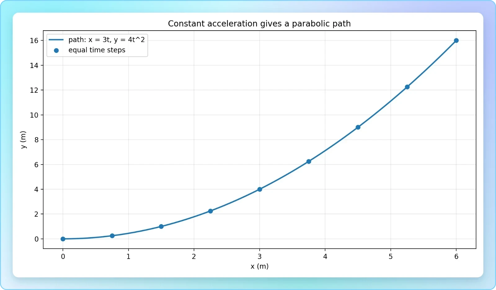
The analytic second derivative of this position function is a constant ##(0\hat{i} + 8\hat{j})\ \text{m/s}^2##, and the numerical routine reproduces it to within rounding error. This agreement illustrates a deeper point: constant acceleration produces a parabolic position curve, exactly the shape traced by projectiles. The next lesson formalises this connection into the standard equations of motion.

Common Misconceptions and Preparing for Equations of Motion

Several persistent misconceptions surround two-dimensional acceleration, and naming them explicitly helps learners avoid them. The most common is the belief that acceleration necessarily implies a change in speed, which the perpendicular case decisively refutes. A second is the assumption that acceleration must point in the direction of motion, which holds only for straight-line travel.

Diagnosing Frequent Errors

Another frequent error is treating acceleration as a scalar and adding magnitudes without regard to direction. Vectors must be combined component by component, and ignoring direction produces answers that are numerically plausible but physically wrong. Careful sign discipline and a clear diagram prevent most of these mistakes before they arise.

Learners also sometimes confuse average and instantaneous acceleration, applying an interval average as though it described every moment within the interval. When acceleration varies, the average conceals that variation entirely. Always ask whether the quantity required is an interval summary or a moment-by-moment description before selecting a formula.

Bridging to the Next Lesson

With acceleration established as a vector and its components understood, the stage is set for the constant-acceleration equations in two dimensions. Those equations apply separately along each axis, linked only by the shared time variable. Everything derived here becomes the input to that next step, so fluency with components is the essential prerequisite.

The habit of decomposing vectors, checking directions, and distinguishing speed from velocity will serve throughout projectile and circular motion analysis. Each later lesson assumes these skills are automatic. Revisiting the worked example and the component tables above is a sound way to consolidate before advancing to the formal equations of motion.