Position, Displacement, and Velocity Vectors

Motion in a plane becomes genuinely tractable the moment we stop treating position, displacement, and velocity as loose collections of numbers and start treating them as single geometric objects. In one dimension, a sign was enough to encode direction; in two dimensions, direction lives in an angle, and magnitude lives in a length. This lesson, the sixth in a thirty-part course on two-dimensional kinematics, builds that bridge carefully. It assumes you can already add and subtract vectors and scale them by numbers, and it prepares you for the acceleration vector that follows.

The central idea is deceptively simple: every quantity that answers "where" or "how fast, and which way" is a vector, and every vector in a plane can be written as a pair of components. Once position is a vector, displacement becomes a difference of vectors, and velocity becomes a displacement divided by an interval of time. That chain of definitions is the backbone of everything from projectile arcs to satellite orbits, and it deserves to be built slowly and precisely rather than memorised as formulas.

Throughout, we will keep one eye on physical meaning and one eye on computation. A runner rounding a bend, a drone hovering against a crosswind, and a ball arcing toward a hoop all obey the same three definitions. By the end of this lesson you should be able to write a position vector, compute a displacement vector between two instants, and derive an average or instantaneous velocity vector, with confidence in both the algebra and the geometry.

Position as a Vector: Locating a Particle in the Plane

Position answers a single question: relative to a chosen origin, where is the object right now? In two dimensions that answer requires two independent pieces of information, and the cleanest way to package them is a position vector drawn from the origin to the particle. The vector carries both the distance from the origin and the direction of that line, so it encodes location completely.

Coordinates, Components, and the Position Vector

Choose a Cartesian frame with origin ##O## and unit vectors ##\hat{i}## and ##\hat{j}## along the axes. A particle at coordinates ##(x, y)## has position vector ##\vec{r} = x\hat{i} + y\hat{j}##. The components are signed numbers, so a point in the third quadrant simply has negative ##x## and negative ##y## components, and no special cases are needed.

The magnitude of the position vector, ##|\vec{r}| = \sqrt{x^2 + y^2}##, is the straight-line distance from the origin, while its direction is the angle measured from the positive ##x##-axis. That angle is usually written ##\theta = \tan^{-1}(y/x)##, with a quadrant correction applied whenever ##x## is negative, because the inverse tangent alone cannot distinguish opposite directions.

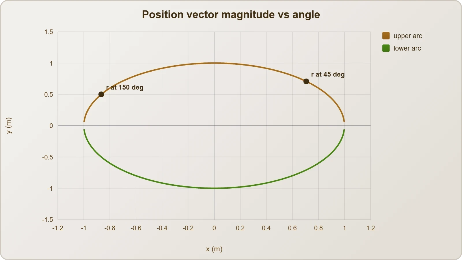
Notice that the position vector is a function of time. As the particle moves, both components change, and the tip of the vector traces out the trajectory in the plane. This is a powerful mental picture: the path of a moving object is literally the curve swept by the head of its position vector as ##t## advances.

Choosing an Origin and Reading the Frame

The origin is a human choice, not a physical absolute. Shifting the origin changes every position vector by the same constant vector, yet leaves displacements and velocities untouched. That invariance is why problems can be solved in whichever frame makes the algebra shortest, and why the choice of origin should be stated explicitly at the start of any calculation.

In practice, examiners and textbooks favour origins at the launch point of a projectile, the centre of a circular track, or the initial location of a moving body. Each choice simplifies one part of the mathematics. The skill being tested is not memorising a preferred origin but recognising which frame turns a messy expression into a clean one.

Displacement: The Vector Change in Position

Displacement is the vector that takes a particle from one position to another. If the particle sits at ##\vec{r}_1## at time ##t_1## and at ##\vec{r}_2## at time ##t_2##, the displacement is the difference ##\Delta\vec{r} = \vec{r}_2 - \vec{r}_1##. Because it is built from a vector subtraction, it inherits the rules you practised in the previous lesson.

Computing Displacement from Two Positions

In components, the subtraction is performed axis by axis: ##\Delta x = x_2 - x_1## and ##\Delta y = y_2 - y_1##. The order matters, since reversing the two instants flips the sign of the whole vector. Displacement therefore points from the earlier position toward the later one, never the other way round.

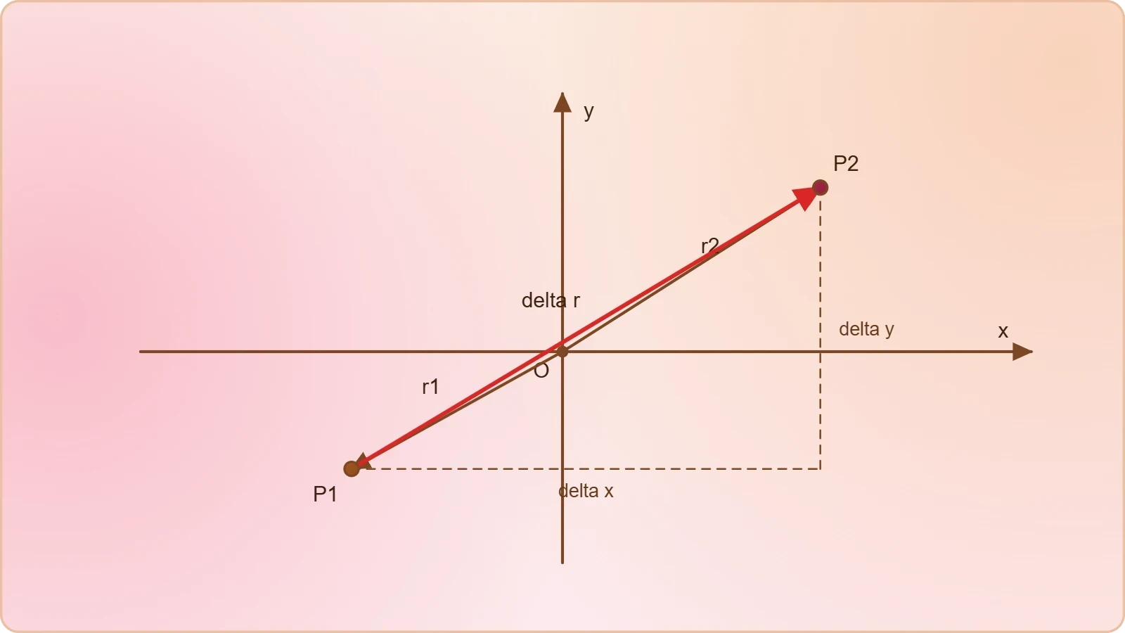
The magnitude ##|\Delta\vec{r}| = \sqrt{(\Delta x)^2 + (\Delta y)^2}## is the straight-line separation between the two points, not the distance actually travelled along the path. A runner who completes a full lap of a track has covered a large distance but has zero displacement, because the start and end points coincide.

This distinction between distance and displacement is one of the most frequently examined ideas in introductory kinematics. Distance is a scalar that accumulates along the path; displacement is a vector that depends only on the endpoints. Confusing the two leads directly to incorrect velocity calculations, so it is worth stating plainly and often.

Geometric Interpretation and Independence from the Origin

Geometrically, displacement is the arrow drawn from the tip of ##\vec{r}_1## to the tip of ##\vec{r}_2##. If you shift the origin, both position vectors change by the same constant, and that constant cancels in the subtraction. Displacement is therefore independent of where the observer places the origin, which is exactly what a physical quantity should be.

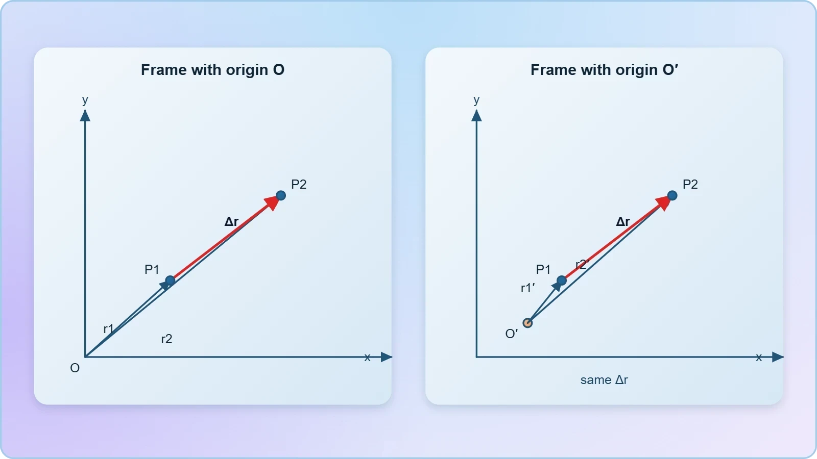
This cancellation is a small but important lesson in vector algebra. It shows that differences of vectors are more physically meaningful than the vectors themselves, and it foreshadows the derivative, where an infinitesimal displacement will be divided by an infinitesimal time interval to produce velocity.

Average Velocity as a Vector Quotient

Average velocity is the displacement divided by the time interval over which it occurred. Written as a vector equation, ##\vec{v}_{avg} = \Delta\vec{r} / \Delta t##, it inherits both the direction of the displacement and a magnitude measured in metres per second. It is a vector quotient in the sense that a vector is divided by a scalar, which simply scales the vector.

Direction, Magnitude, and the Meaning of the Average

Because the numerator is a vector and the denominator is a positive scalar, the average velocity points in exactly the same direction as the displacement. Its magnitude is the straight-line separation divided by the elapsed time, which is generally smaller than the average speed whenever the path curves or doubles back.

Average speed, by contrast, is total distance divided by total time, a scalar with no directional information. On a straight path traversed without reversal the two coincide, but on any curved trajectory they diverge. Examiners exploit this gap constantly, so always check whether a question asks for speed or for velocity before substituting numbers.

The component form is often the fastest route to an answer. Compute the two component displacements, divide each by the same time interval, and you have the two components of average velocity. The magnitude and direction then follow from the usual Pythagorean and inverse-tangent relations applied to those components.

Worked Example: A Drone Crossing a Field

Suppose a drone moves from ##(2, 1)## metres to ##(14, 9)## metres in four seconds. The displacement is ##12\hat{i} + 8\hat{j}## metres, so the average velocity is ##3\hat{i} + 2\hat{j}## metres per second. Its magnitude is ##\sqrt{13} \approx 3.61## m/s, directed at about ##33.7^\circ## above the horizontal.

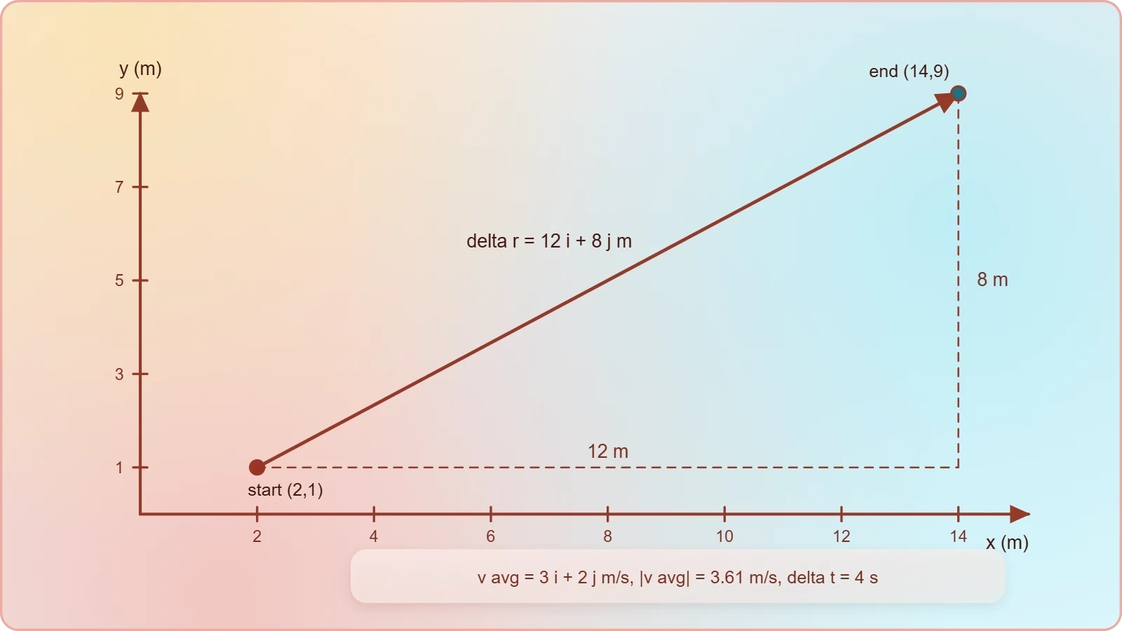
Notice how the arithmetic stays clean when the components are handled separately. Mixing the axes, or dividing the magnitude of the displacement by time without checking direction, produces answers that look plausible but fail the physical test. Component discipline is the single most reliable habit in two-dimensional kinematics.

Instantaneous Velocity and the Tangent Limit

Average velocity over a long interval hides the details of the motion. To capture what happens at a single instant, we shrink the time interval toward zero and take the limit. The result is the instantaneous velocity, the derivative of the position vector with respect to time, and it points along the tangent to the trajectory at that moment.

From Difference Quotient to Derivative

Formally, ##\vec{v} = \lim_{\Delta t \to 0} \Delta\vec{r}/\Delta t = d\vec{r}/dt##. Because differentiation is linear, it acts on each component separately, giving ##v_x = dx/dt## and ##v_y = dy/dt##. The vector velocity is then reassembled from these two scalar derivatives.

This is where the calculus of the course begins to pay off. If the position components are known as functions of time, the velocity components follow by straightforward differentiation. Conversely, integrating the velocity components recovers the position, up to a constant vector fixed by the initial conditions.

The direction of the instantaneous velocity is the direction of motion at that instant, which is why it is always tangent to the path. On a curved trajectory the tangent direction changes continuously, and that changing direction is precisely what the next lesson will formalise as acceleration.

Speed Versus Velocity in the Instantaneous Limit

Instantaneous speed is the magnitude of the instantaneous velocity vector, ##|\vec{v}|##, and it is always non-negative. Unlike average speed, which can differ sharply from the magnitude of average velocity, instantaneous speed and the magnitude of instantaneous velocity are identical by definition. That identity is a useful sanity check in calculations.

A car travelling at a steady sixty kilometres per hour around a bend has constant speed but changing velocity, because the direction of the velocity vector rotates. This single example captures the essential difference between the scalar and vector descriptions, and it prepares the ground for centripetal acceleration later in the course.

Working in Components: A Computational Workflow

Most errors in two-dimensional kinematics come from skipping the component step and trying to reason with magnitudes and angles directly. A disciplined workflow avoids this: resolve every vector into components, perform the algebra axis by axis, then reassemble the result. The method is mechanical, which is precisely why it is reliable under examination pressure.

A Step-by-Step Procedure with Code

Begin by writing the position vectors at the two instants in component form. Subtract to obtain the displacement, divide by the time interval to obtain average velocity, and finally compute magnitude and direction. Each step is a small, checkable calculation, and the final answer can be verified by substituting back into the original definitions.

When the position is given as a function of time rather than as discrete points, the same workflow applies with differentiation replacing subtraction. The code below performs both routes for a particle whose coordinates are quadratic in time, which is exactly the form produced by constant acceleration in each axis.

import numpy as np

def position(t):
    # coordinates in metres as functions of time in seconds
    x = 2.0 + 3.0 * t
    y = 1.0 + 4.0 * t - 0.5 * 9.81 * t**2
    return np.array([x, y])

t1, t2 = 0.0, 2.0
r1, r2 = position(t1), position(t2)
displacement = r2 - r1
avg_velocity = displacement / (t2 - t1)

# instantaneous velocity by numerical differentiation
dt = 1e-6
v_inst = (position(t2 + dt) - position(t2 - dt)) / (2 * dt)

print("displacement:", displacement)
print("average velocity:", avg_velocity)
print("instantaneous velocity:", v_inst)
print("speed:", np.linalg.norm(v_inst))

Running this snippet for the stated functions returns a displacement of ##(6, -11.62)## metres and an average velocity of ##(3, -5.81)## metres per second. The instantaneous velocity at two seconds is ##(3, -15.62)## metres per second, reflecting the downward acceleration of gravity in the vertical component.

Common Pitfalls and How to Avoid Them

The first pitfall is treating the magnitude of a displacement as a distance travelled; the second is forgetting that the time interval must be positive when dividing. The third, and most damaging, is mixing units between axes, such as metres in one component and centimetres in the other. Consistent SI units eliminate an entire class of errors.

A fourth pitfall is rounding intermediate results too early. Keep full precision through the component calculations and round only the final magnitude and angle. A fifth is ignoring the quadrant when computing the direction angle, which silently produces answers that point in the wrong direction by one hundred and eighty degrees.

Physical Insight: Reading Motion from Vectors

Vectors are not merely a bookkeeping device; they carry the physical story of the motion. The position vector locates the particle, the displacement vector records the net change, and the velocity vector describes the instantaneous rate and direction of that change. Reading these three together gives a complete kinematic description at any moment.

Trajectories, Tangents, and the Shape of Motion

As the particle moves, the tip of the position vector traces the trajectory, and the velocity vector is always tangent to that curve. Where the tangent is horizontal, the vertical velocity component vanishes, which is exactly the condition for the highest point of a projectile arc. Such geometric observations often replace lengthy algebra.

For uniform circular motion, the position vector has constant magnitude while its direction rotates steadily. The velocity vector remains perpendicular to the position vector throughout, a fact that follows directly from differentiating ##\vec{r}\cdot\vec{r} = R^2## with respect to time. This perpendicularity is the seed of centripetal acceleration.

That short derivation is worth pausing over. It shows that a constant distance from the origin forces the velocity to be perpendicular to the position, without any appeal to geometry diagrams. Results of this kind demonstrate why the vector formulation is more than convenient notation; it generates physical insight almost automatically.

Preparing for Acceleration in Two Dimensions

The next lesson extends the same logic to acceleration, defined as the derivative of velocity with respect to time. Just as velocity measures how position changes, acceleration measures how velocity changes, and in two dimensions a change of direction alone is enough to produce a non-zero acceleration. That is the conceptual leap waiting in Lesson Seven.

Before moving on, consolidate the three definitions in this lesson and practise switching between component form and magnitude-angle form. Fluency in that translation is the prerequisite for projectile problems, where horizontal and vertical motions are analysed independently, and for circular motion, where the velocity direction rotates continuously.