On This Page
Understanding the Principle of Homogeneity
The Fundamental Statement
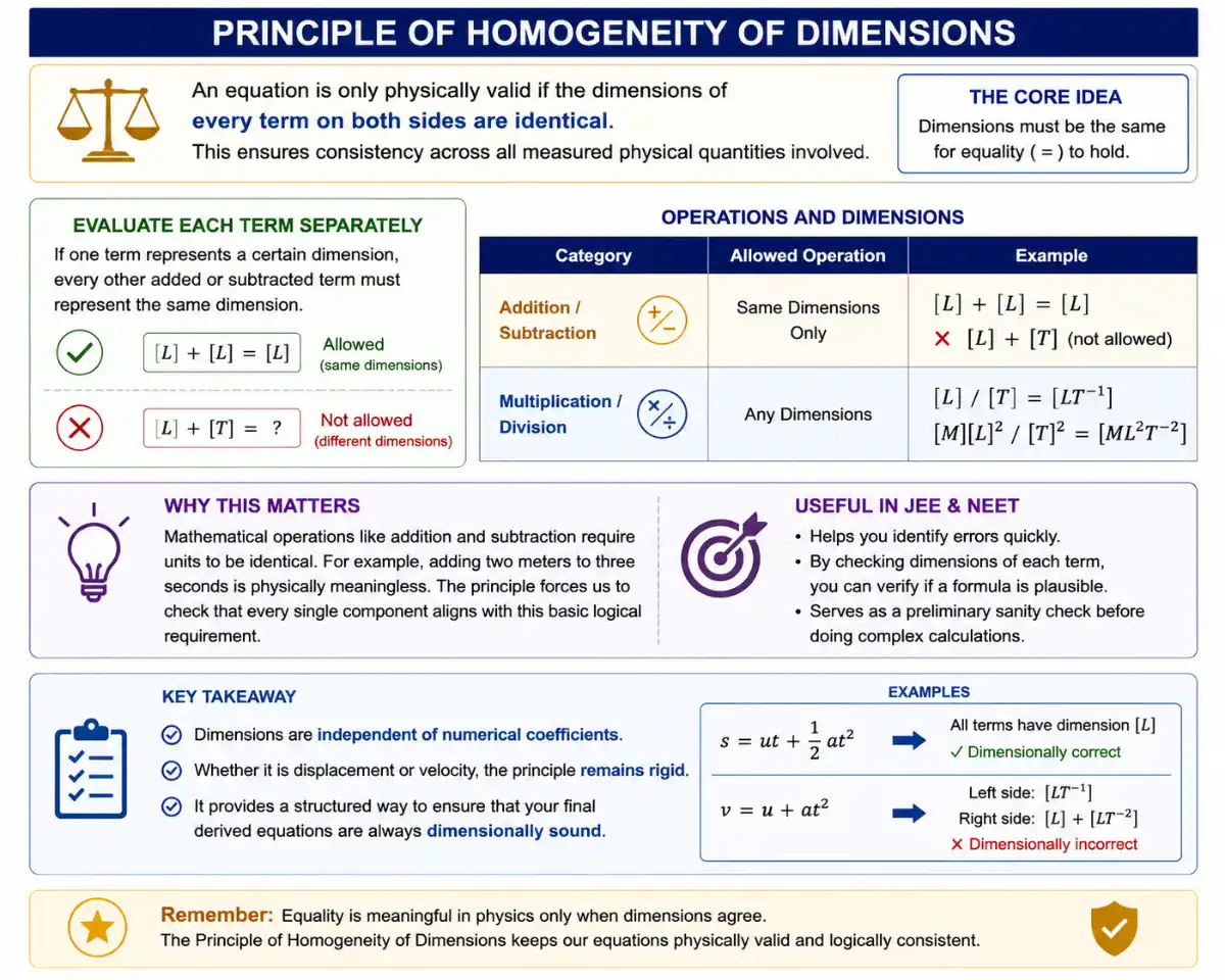
The Principle of Homogeneity of Dimensions is a cornerstone of physics. It asserts that an equation is only physically valid if the dimensions of every term on both sides are identical. This ensures consistency across all measured physical quantities involved.
When you encounter a physical expression, you must evaluate each term separately. If one term represents length, every other added or subtracted term must also represent length. You cannot add a mass unit to a time unit in physics.
| Category | Allowed Operation | Example |
|---|---|---|
| Addition/Subtraction | Same Dimensions Only | [L] + [L] = [L] |
| Multiplication/Division | Any Dimensions | [L] / [T] = [LT⁻¹] |
Mathematical operations like addition and subtraction require units to be identical. For example, adding two meters to three seconds is physically meaningless. The principle forces us to check that every single component aligns with this basic logical requirement.
In JEE and NEET, this concept helps you identify errors quickly. By checking the dimensions of each term, you can verify if a formula is plausible. It serves as a preliminary sanity check before performing any complex algebraic calculations.
Always remember that dimensions are independent of the numerical coefficients. Whether you are dealing with displacement or velocity, the principle remains rigid. It provides a structured way to ensure that your final derived equations are always dimensionally sound.
Why Dimensional Consistency Matters
Consistency is vital because physics describes real-world phenomena. If an equation lacks dimensional homogeneity, it fails to model reality accurately. This principle prevents us from combining incompatible quantities, which would lead to nonsensical results in any scientific experiment.
Consider a simple expression where you calculate total energy. If you add kinetic energy to potential energy, both must share the same dimensions of work. Any discrepancy suggests a flaw in the derivation or an incorrect understanding of variables.
This rule also simplifies complex problems significantly. By focusing on the dimensions rather than the values, you can narrow down potential answers. It acts as a powerful analytical tool that saves time during competitive exams like the JEE.
Students often overlook this requirement when working with constants. However, constants must also possess the correct dimensions to balance the equation. If a constant is missing, the equation will be dimensionally unbalanced, signaling an error in your logic.
By enforcing this standard, scientists ensure that laws are universal. Whether measured in SI or CGS, the dimensional consistency holds true. This universality is what allows physicists to translate findings across different systems of measurement without losing meaning.
Verifying Physical Equations
Analyzing Kinematic Equations
Let us examine the classic kinematic equation ##s = ut + \dfrac{1}{2}at^2##. According to the principle, each term must have the same dimensions as distance. We verify this by calculating the individual dimensions for every term in the expression.
The first term is displacement ##s##, which has dimensions ##[L]##. The second term is ##ut##, where velocity ##[LT^{-1}]## is multiplied by time ##[T]##. This results in ##[L]##, matching the displacement term perfectly as required by the rule.
The final term is ##\dfrac{1}{2}at^2##. Acceleration ##[LT^{-2}]## multiplied by time squared ##[T^2]## yields ##[L]##. Since all three terms possess the dimension of length, the equation is dimensionally correct. This confirms the validity of the kinematic relation.
![An instructional diagram outlining the process of dimensional analysis using the classic kinematic equation s = ut + (1/2)at^2. It lists each term (displacement, velocity x time, and acceleration x time^2) and calculates their dimensions to show that all terms equate to the dimension of length [L], rendering the equation valid. A counter-example of an invalid equation (s = ut + at) is provided, along with key takeaways highlighting that every term in an equation must have identical dimensions.](https://jupiterscience.com/wp-content/uploads/2026/06/principle-of-homogeneity-of-dimensions-description-teach-the-principle-that-only-quantities-with-th-1.webp)
This verification process is essential for all physics students. When you derive new formulas, always apply this check. It prevents common mistakes where powers of time or length are accidentally omitted during the derivation of complex physical motion equations.
Even if the numerical factor ##1/2## is invisible to dimensional analysis, the variables must align. If the expression were ##s = ut + at##, it would fail the test because ##at## has dimensions of velocity, not length. Always check.
Handling Transcendental Functions
Transcendental functions like ##\sin(x)##, ##\cos(x)##, and ##e^x## introduce unique constraints. The argument ##x## within these functions must always be dimensionless. This is because you cannot take the sine of a physical quantity like mass or time directly.
If you see a term like ##\sin(kx)##, the product ##kx## must be a pure number. This implies that the dimensions of ##k## are the inverse of the dimensions of ##x##. This is a common pattern in wave equations.
Exponential functions follow similar rules. In ##e^{-at}##, the exponent ##at## must be dimensionless. Therefore, the constant ##a## must have dimensions of inverse time ##[T^{-1}]##. This is critical for solving problems involving decay or growth rates in physics.
Logarithmic functions also require dimensionless arguments. If you encounter ##\ln(P/P_0)##, the ratio ##P/P_0## must be dimensionless. This confirms that ##P## and ##P_0## share identical dimensions, such as pressure or density. This rule is absolute in all physics calculations.
Failing to account for these constraints will lead to incorrect conclusions. Always verify the arguments of these functions during your board exams. It is a frequent point of testing for examiners to see if students understand these subtle rules.
Limitations and Advanced Applications
Dimensional Correctness vs. Reality
A major limitation is that dimensional homogeneity does not guarantee a formula is physically correct. An equation might be dimensionally consistent but still contain incorrect numerical constants. For example, ##s = ut + at^2## is dimensionally consistent but physically wrong.
The principle cannot determine the value of dimensionless constants. Whether the coefficient is ##1##, ##1/2##, or ##2\pi##, dimensional analysis remains blind to these factors. You must use physical laws or experimental data to find these precise numerical values correctly.
Furthermore, the principle cannot distinguish between different physical quantities that share the same dimensions. Work, energy, and torque all have the same dimensional formula ##[ML^2T^{-2}]##. The principle will not flag an equation if you swap energy for torque.
This means you must supplement dimensional analysis with conceptual knowledge. Do not rely solely on dimensions to derive formulas. Always verify the physical context of the problem to ensure that the chosen quantities actually make sense in that application.
Despite these limitations, the method is indispensable. It acts as a primary filter to discard clearly impossible equations. When used in conjunction with other methods, it becomes the most robust tool for checking your work in complex physics problems.
Applying the Principle in Electricity
In electricity, the principle is just as rigorous. Consider Ohm’s Law: ##V = IR##. We check the dimensions of potential difference against current multiplied by resistance. This ensures the relationship between voltage, current, and resistance is always logically consistent.
Potential difference ##V## has dimensions ##[ML^2T^{-3}A^{-1}]##. Current ##I## is ##[A]##. Resistance ##R## is ##[ML^2T^{-3}A^{-2}]##. Multiplying ##I## and ##R## gives ##[A] \times [ML^2T^{-3}A^{-2}] = [ML^2T^{-3}A^{-1}]##. The dimensions match perfectly on both sides of the equation.
This consistency is crucial when dealing with complex circuits. Whether you are calculating impedance or power dissipation, the principle guides you. It prevents the common error of adding resistance to reactance without considering their complex phase relationships correctly.
You can also use this to derive units for unknown constants in electromagnetic equations. If you know the dimensions of force and charge, you can determine the dimensions of the electric field. This is a very common JEE question.
Always maintain a habit of checking these electrical units. By doing so, you avoid errors when solving for unknowns in circuit diagrams. It is a simple step that ensures your physical model of the electrical system is correct.
Problem Solving and Practice
Common Errors to Avoid
Students frequently make the mistake of ignoring coefficients. While coefficients are dimensionless, they are part of the equation's structure. You must ensure the entire expression, including all terms, respects the homogeneity of dimensions before finalizing your exam answers.
Another error is confusing the unit with the dimension. A unit depends on the system, like meters or centimeters, but the dimension remains ##[L]##. Never mix units and dimensions in the same equation; keep your notation clear and consistent.
Many students forget to apply the principle to exponents and arguments of trigonometric functions. These must be dimensionless, yet they are often missed. Always perform a quick check on these parts of the equation during your final review.
Avoid the trap of thinking that dimensional correctness equals absolute truth. Always verify the physics behind the equation. If the formula contradicts a known law of nature, it is incorrect, even if it passes the dimensional homogeneity test perfectly.
Finally, practice is the key to mastery. Solve various problems involving mechanics, optics, and thermodynamics. The more you apply the principle, the more intuitive it becomes. This habit will significantly improve your accuracy in competitive physics examinations globally.
| Common Pitfall | Corrective Action |
|---|---|
| Ignoring Coefficients | Verify variables independently |
| Mixing Units/Dimensions | Standardize to [M], [L], [T] |
| Trig/Log Arguments | Ensure they are dimensionless |
Structured Learning Table
To summarize, the principle applies across all domains of physics. Whether you are dealing with basic mechanics or advanced electromagnetism, the requirements remain identical. Use the table below to organize your understanding of these critical dimensional relationships and constants.
| Quantity | Formula | Dimensions |
|---|---|---|
| Force | ##ma## | ##[MLT^{-2}]## |
| Work | ##Fs## | ##[ML^2T^{-2}]## |
| Pressure | ##F/A## | ##[ML^{-1}T^{-2}]## |
This table illustrates how derived units are built from base quantities. Notice how each formula respects the homogeneity of dimensions. By breaking down complex quantities into base dimensions, you can easily verify the consistency of any physical equation encountered.
The example above shows how to find dimensions of a constant like ##G##. By rearranging the formula and applying the principle, you isolate the unknown dimensions. This method is highly effective for solving problems involving universal physical constants today.
Consistent practice with these derivations builds confidence. As you progress through your curriculum, the ability to check equations becomes second nature. This skill is a hallmark of a proficient physics student and a successful candidate for competitive exams.
RESOURCES
- Principle of Homogeneity - Dimensional Analysis Physics - YouTubeyoutube.comDec 17, 2012 ... http://itsmyacademy.com/dimensional-analysis-physics-videos/ This Physics Lesson States & describes the "Principle of Homogeneity" ...
- Why is the principle of homogeneity (units and dimensions) not ...reddit.comApr 4, 2024 ... In the reals, one can show that Cauchy completeness is equivalent to the Least Upper Bound property; does this hold…
- Towards a principle of homogeneity in the field of legal remedies?kluwerlawonline.comView Bridging the gap between Community and national laws: Towards a principle of homogeneity in the field of legal remedies? by - Common Market…
- Homogeneity (physics) - Wikipediaen.wikipedia.orgIn physics, a homogeneous material or system has the same properties at every point; it is uniform without irregularities.
- Principle of Homogeneity of Dimensions Explained - Vedantuvedantu.comThe principle of homogeneity of dimensions states that in any physical equation, the dimensions of each term on both sides must be identical. This…
- Homogeneity Principles in Physics | PDF | Force - Scribdscribd.comThe document discusses the Principle of Homogeneity, which states that dimensions and units of terms in equations must match. It includes various problems ...
- Unit Conversion and Dimensional Analysis - BYJU'Sbyjus.comPrinciple of Homogeneity states that dimensions of each of the terms of a dimensional equation on both sides should be the same. This principle…
- Using the principle of homogeneity of dimensions, which of ... - Allenallen.inTo solve the problem using the principle of homogeneity of dimensions, we need to analyze each of the given equations and check if both…
- what is the basis of principle of homogeneity - Brainly.inbrainly.inMay 28, 2019 ... The principle of homogeneity is that the dimensions of each the terms of a dimensiional equation on both sides are…
- State the principle of homogeneity of dimensions. - Filoaskfilo.comOct 12, 2025 ... The principle of homogeneity of dimensions states that in any physical equation, the dimensions of the terms on both sides…
- Principle of homogeneity | mathematics - Britannicabritannica.comMay 1, 2026 ... Viète retained the classical principle of homogeneity, according to which terms added together must all be of the same dimension.
- Re-Thinking Homogeneity: The Biblical Case for Multi-Ethnic ...9marks.orgSep 25, 2015 ... The “homogeneous unit principle” of church growth has been unquestioningly assumed as the most effective way to multiply disciples and…
- PRINCIPLE OF HOMOGENEITY #physics - Facebookfacebook.comFeb 21, 2026 ... What is the Principle of Homogeneity? In any correct physical equation, the dimensions of all terms on both sides must…
- What is principle of homogeneity in dimension - Brainly.inbrainly.inMar 12, 2024 ... The principle of dimensional homogeneity states that the dimensions of each term in a dimensional equation must be the same…
- Testing the Copernican principle by constraining spatial homogeneityarxiv.orgSep 18, 2012 ... Abstract:We present a new programme for placing constraints on radial inhomogeneity in a dark-energy dominated universe.
0 Comments