On This Page
The Role of Graphs in Experimental Physics
Understanding Graphical Representation
Graphs translate raw experimental data into a visual format that reveals underlying physical trends. By plotting independent variables on the x-axis and dependent variables on the y-axis, researchers identify patterns. These visual representations simplify complex sets of numerical measurements significantly.
| Component | Function | Importance |
|---|---|---|
| X-Axis | Independent Variable | Control parameter |
| Y-Axis | Dependent Variable | Measured outcome |
| Error Bars | Uncertainty Range | Data reliability |
Choosing the correct scale for axes ensures that data remains readable and accurate. A well-chosen scale prevents distortion of the relationship between variables. Students must learn to select intervals that cover the entire range of observed data points clearly.
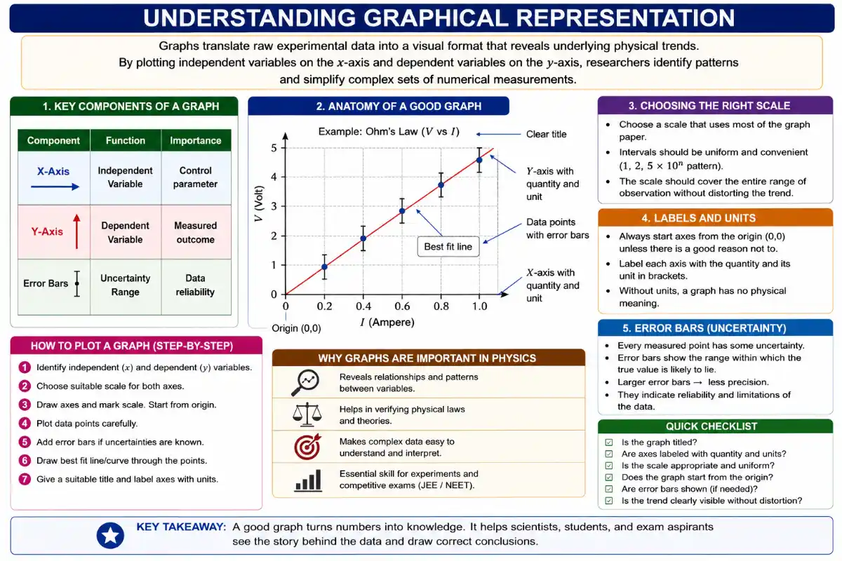
The origin point serves as a reference for all measurements taken during an experiment. Properly labeling axes with the correct units is vital for maintaining dimensional consistency. Without units, a graph lacks physical meaning and cannot represent real phenomena.
Error bars indicate the uncertainty associated with every measured data point in an experiment. These bars provide a visual range where the true value likely exists. Including them helps students appreciate the limitations and precision of their physical measurements.
Physics relies on the relationship between variables to define laws. Whether observing motion or electrical current, graphs allow scientists to verify these laws. Mastering this skill is a fundamental requirement for success in competitive exams like JEE or NEET.
Selecting Proper Axes and Scales
The independent variable belongs on the horizontal x-axis, while the dependent variable occupies the vertical y-axis. This standard convention ensures consistency across all scientific disciplines. Following this rule allows for accurate interpretation of the resulting curve or line.
Scaling requires careful consideration to ensure the graph occupies the available space efficiently. If the scale is too small, the data appears cramped and difficult to analyze. Conversely, an overly large scale makes the graph impossible to interpret.
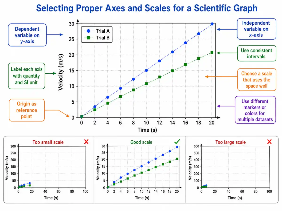
Each axis must clearly state the physical quantity being measured along with its respective SI unit. For example, plotting velocity in meters per second requires specific labeling. Omitting these details leads to confusion and errors in final data analysis.
Consistent intervals on axes maintain the proportionality of the plotted data throughout the experiment. Avoid using broken scales unless absolutely necessary, as they can misrepresent trends. A clean, linear scale is always preferred for accurate slope and intercept determination.
When comparing multiple datasets on one graph, use distinct markers or colors. This practice clarifies the relationship between different physical conditions. Clear presentation is just as important as the mathematical accuracy of the data points plotted during experiments.
Analyzing Slopes and Intercepts
The Meaning of Physical Slope
The slope of a linear graph represents the rate of change between two physical quantities. Mathematically, it is defined as the ratio of the change in y to the change in x. This value often carries significant physical meaning.
| Graph Plot (Y vs X) | Slope Represents | Unit |
|---|---|---|
| Force vs Extension | Spring Constant (k) | N/m |
| Voltage vs Current | Resistance (R) | Ohms |
| Velocity vs Time | Acceleration (a) | m/s² |
To calculate the slope, select two distinct points on the straight line. Apply the standard formula ##m = \dfrac{y_2 - y_1}{x_2 - x_1}## to determine the gradient. Ensure that the units of the slope match the quotient of the y and x units.
In kinematics, a velocity-time graph features a slope equal to acceleration. The units of this slope are meters per second squared, which is the standard unit for acceleration. This reveals how graphs directly link to basic physical motion concepts.
The dimension of the slope is derived from the dimensions of the variables on the axes. If the y-axis represents force and the x-axis represents extension, the slope represents a stiffness constant. Dimensional consistency is a key analytical check.
Students should practice calculating slopes from various types of experimental data. Being able to extract constants from a slope is a frequent requirement in advanced physics. This skill transforms a simple line into a powerful tool for discovery.
Consider a spring experiment where force is plotted against extension. The slope of this line corresponds to the spring constant ##k##. If force is measured in Newtons and extension in meters, the slope unit is clearly Newtons per meter.
To find the slope, choose two points far apart on the line. Using distant points reduces the impact of small reading errors on the final result. Always maintain precision by using the highest possible accuracy for your coordinate selection.
The intercept represents the value of the dependent variable when the independent variable is zero. It may indicate a systematic error or a specific initial condition. Identifying the intercept is essential for constructing the correct equation of the line.
The general equation for a line is ##y = mx + c##, where ##m## is the slope and ##c## is the intercept. Understanding this equation allows students to predict outcomes for values outside the measured range of their experiment.
Advanced problems often require manipulating these graphs to find unknown parameters. By comparing experimental results to theoretical models, students confirm the validity of their measurements. This iterative process is the heart of experimental physics in academic research settings.
Area Under the Curve
Interpreting Graphical Areas
The area under a curve represents the integral of the vertical variable with respect to the horizontal variable. In physics, this calculation often results in a new physical quantity. It is a fundamental method for analyzing cumulative experimental effects.
For a velocity-time graph, the area under the line represents the total displacement. Since velocity is ##\dfrac{dx}{dt}##, the area ##\int v dt## gives the change in position. This relationship is vital for solving complex problems in classical mechanics.
When calculating area, ensure that the units are multiplied correctly. If the y-axis is in Newtons and the x-axis is in meters, the area represents work done in Joules. This dimensional analysis confirms the physical meaning of the result.
For non-linear graphs, the area is calculated using segments or integration techniques. Students must be comfortable with these mathematical tools to handle advanced physics problems. Approximating area using small rectangles is a common, reliable approach for experimental data sets.
The ability to interpret area is particularly useful in thermodynamics and electromagnetism. Whether calculating work done by a gas or magnetic flux, the graphical approach provides clarity. It bridges the gap between abstract calculus and tangible physical experimental outcomes.
Practical Applications of Area
| Graph Type | Area Represents | Units |
|---|---|---|
| Velocity-Time | Displacement | meters |
| Force-Position | Work | Joules |
| Current-Time | Charge | Coulombs |
The table above summarizes key graphical relationships frequently encountered in exams. Memorizing these connections saves time and prevents errors during high-pressure testing. Each entry demonstrates how physical integration links two distinct quantities through the concept of area calculation.
In a force-position graph, the area represents the energy transferred to an object. This is a core concept in the study of work, energy, and power. Students should visualize the area as the accumulation of force over a specific distance.
Consider the current-time graph used in electrical experiments. The area under this curve corresponds to the total electric charge passed through a circuit. This relationship is essential for understanding capacitor charging cycles and other time-dependent electrical phenomena effectively today.
Every area calculation must be checked for dimensional correctness. If the result does not match the expected units of the quantity, re-examine the axes. Proper attention to units ensures that the physical interpretation of the graphical area remains valid.
Mastering these interpretations allows students to tackle complex multi-step problems with confidence. By recognizing the physical significance of an area, one can bypass tedious algebraic derivations. This efficient approach is highly valued in competitive exams like JEE Advanced level.
Advanced Graphical Techniques
Pendulum and Ohm's Law Graphs
The simple pendulum experiment often involves plotting ##T^2## against length ##l##. The resulting graph is a straight line passing through the origin. The slope of this line allows for the calculation of the local acceleration due to gravity.
Ohm's Law is demonstrated by plotting voltage against current. A linear graph confirms the resistance as a constant. The slope of this ##V-I## plot is exactly equal to the resistance ##R##, measured in Ohms as a standard unit.
These classic experiments teach students how to verify theoretical laws using empirical data. When the experimental points do not fall perfectly on the line, we use the line of best fit. This technique accounts for random errors in measurements.
The line of best fit minimizes the vertical distance between the data points and the line. It provides the most accurate estimation of the slope and intercept. This statistical approach is crucial for reporting reliable results in any physics laboratory.
Both the pendulum and Ohm’s law experiments serve as foundational exercises for students. They illustrate how theory and experiment converge through graphical representation. Understanding these specific graphs prepares learners for more complex analytical tasks in future engineering studies.
In the pendulum experiment, the period ##T## is related to length ##l## by ##T = 2\pi \sqrt{\dfrac{l}{g}}##. Squaring both sides yields ##T^2 = \dfrac{4\pi^2}{g} \cdot l##. By plotting ##T^2## versus ##l##, we obtain a slope equal to ##\dfrac{4\pi^2}{g}## for analysis.
To find the value of ##g##, simply calculate the slope of the line and rearrange the equation. This method demonstrates how graphical analysis simplifies the extraction of physical constants. It is a standard procedure in many undergraduate physics laboratory experiments.
The intercept in this specific plot should theoretically be zero. If a non-zero intercept appears, it suggests a systematic error in the length measurement. Students must learn to diagnose these issues by looking closely at their plotted experimental data.
Accuracy in plotting is paramount for these types of calculations. A slight deviation in the slope leads to a significant error in the calculated gravity. Precision in reading the instruments and plotting the points is the key to success.
Finally, always include units for the calculated constants. Gravity must be expressed in ##m/s^2## to remain physically meaningful. This consistency reinforces the link between mathematical results and the physical reality of the experiment being performed in the lab.
RESOURCES
- Why are gradient and graphs used in labs? - Physics Stack Exchangephysics.stackexchange.comOct 23, 2018 ... Experimental physics also incorporates uncertainty. You can never say the time constant = 3 ms, but it exists as a…
- A guide to Physics paper 6 : r/igcse - Redditreddit.comOct 21, 2024 ... Physics paper 6 is the easiest scoring paper. All of it is memorizing the precautions of an experiment or plotting…
- Quantum Experiments and Graphs: Multiparty States as Coherent ...link.aps.orgDec 15, 2017 ... For that, we first translate the quantum physics question “Which d -dimensional GHZ states can be created?” into the graph…
- I'm really bad at Experimental Physics. Are there any good textbooks ...reddit.comAug 16, 2025 ... Graphs and linear regression is a broad topic. Do you have an example you can post and walk through your…
- [2211.05143] Attention to the strengths of physical interactions - arXivarxiv.orgNov 9, 2022 ... ... graph-based event classification for particle physics experiments. ... (graphs). Our results in event classification show that the ...
- Attention to the strengths of physical interactions: Transformer and ...scipost.orgJul 28, 2025 ... ... graph-based event classification for particle physics experiments. ... (graphs). Our results in event classification show that the ...
- Experimental entanglement of six photons in graph states - Naturenature.comJan 14, 2007 ... Authors and Affiliations. Hefei National Laboratory for Physical Sciences at Microscale and Department of Modern Physics, University of ...
- Experimental Identification of the Second‐Order Non‐Hermitian Skin ...advanced.onlinelibrary.wiley.comNov 13, 2022 ... Physics-graph-informed machine learning (PGIML), formulated by integrating physical principles, graph visualization, and machine learning, ...
- Students' construction of linear and nonlinear qualitative graphs ...iopscience.iop.orgDec 19, 2025 ... Students' construction of linear and nonlinear qualitative graphs corresponding to a hypothetical physics experiment, Condon, Orlaith, ...
- Logger Pro™ 3 - Verniervernier.comDevelop your own experiment files to match your curriculum. Versatile. Supports over 80 Vernier sensors for real-time graphing and analysis. Collect data from a ...
- Experimental Readiness Review Chart | Jefferson Labjlab.orgExperimental Readiness Review Chart · Who is assigned as Physics Division Liaison for the experiment; Installation schedule · Existing equipment requirements ...
- Empirical Force Laws: Gravitational Force Experiment - Physics! Blog!kellyoshea.blogSep 22, 2012 ... Using LinReg makes graphing easier (no more hand-drawn graphs), and it also forces us to think about the range of…
- Non-thesis WIC | Department of Physicsphysics.oregonstate.edu... Experimental Physics along with an additional upper-division physics elective. ... graphs and pictures takes place all through the experiment. You keep an ...
- Investigating the linear equations of maximum and minimum slope ...iopscience.iop.orgThis study investigates the maximum and minimum slope lines of a linear graph used in high school physics experiments.
- Supersymmetric gauge theory on the graph - Oxford Academicacademic.oup.comProgress of Theoretical and Experimental Physics, Volume 2022, Issue 4 ... graph and the dual graph. In the continuous theory, a scalar curvature ...