Superposition Principle and Interference

Sound waves rarely travel alone. In any real acoustic environment — a concert hall, an exam hall with echoing corridors, or a laboratory resonance tube — multiple pressure disturbances overlap continuously, and the resulting field is not the sum of independent experiences but a single, physically measurable pressure history. The superposition principle formalises this: at any point, the instantaneous displacement or pressure equals the algebraic sum of the contributions from each individual wave. For IIT JEE aspirants, this lesson converts that deceptively simple statement into a working analytical instrument.

Building directly on the wave equation and speed of sound established in Lesson 2, this third lesson of thirty examines how two or more sound waves combine, when they reinforce, when they cancel, and how the resulting intensity pattern can be predicted quantitatively. The treatment moves from the general superposition statement to the specific case of interference between coherent sources, then to the intensity distribution, fringe conditions, and the energy-conservation subtleties that examiners frequently probe. Every derivation is tied to a numerical or conceptual question type seen in JEE Main and Advanced papers.

The lesson deliberately stops short of standing waves, which form the subject of Lesson 4, and assumes fluency with the travelling-wave description from Lesson 2. What follows is therefore a bridge: superposition supplies the mathematical machinery, interference supplies the observable phenomenon, and the intensity relations developed here become the foundation for resonance and organ-pipe analysis in the next lesson.

The Superposition Principle as a Linear-System Statement

Superposition is not a universal law of nature; it is a consequence of linearity. The acoustic wave equation is linear in the pressure perturbation, meaning that if two pressure fields each satisfy the equation, their sum does too. This linearity holds for small-amplitude disturbances in air, where density variations remain a tiny fraction of ambient density and nonlinear convective terms are negligible.

The practical implication is significant. A listener at a point in a room receives a pressure signal that is the algebraic sum of every arriving wave, and each wave can be analysed independently before summation. Amplitude, phase, and frequency of each component are preserved in the sum; only the resultant changes. This independence is what makes acoustic analysis tractable at all.

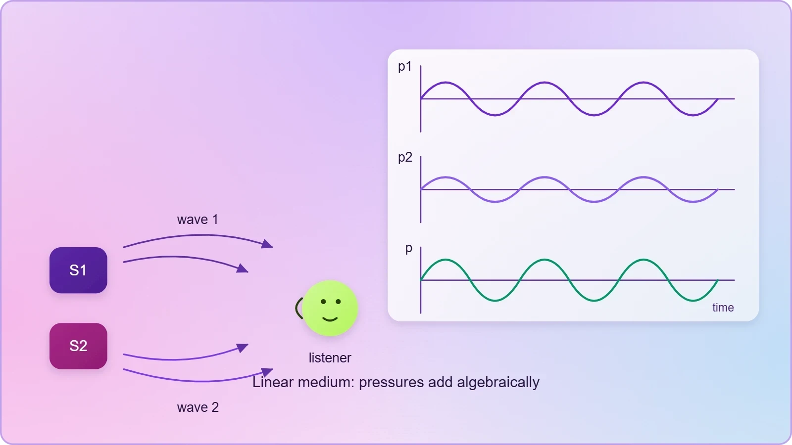
Mathematical formulation for two travelling waves

Consider two sound waves of the same angular frequency ##\omega## travelling along the same line and arriving at a point with a phase difference ##\phi##. Their pressure variations may be written as ##p_1 = p_{01}\sin(\omega t)## and ##p_2 = p_{02}\sin(\omega t + \phi)##. The resultant pressure is their algebraic sum, and the superposition principle guarantees that this sum is itself a harmonic wave of the same frequency.

Applying the standard trigonometric identity for the sum of two sines yields a resultant amplitude that depends on both individual amplitudes and the phase difference. The derivation is worth reproducing because it recurs throughout the syllabus and underpins the intensity relations developed later in this lesson.

Expanding the second term and collecting coefficients of ##\sin(\omega t)## and ##\cos(\omega t)## gives a resultant of the form ##p = A\sin(\omega t + \theta)##, where the resultant amplitude ##A## satisfies the cosine rule relationship below. Note that when ##p_{01} = p_{02} = p_0##, the expression collapses to ##A = 2p_0\cos(\phi/2)##, the canonical interference result.

Phase difference and path difference

In acoustic problems the phase difference is rarely given directly; it must be constructed from geometry. Two coherent sources separated by a distance emit waves that travel different path lengths to a field point, and the path difference ##\Delta x## converts to phase difference through the wavelength. The relation ##\phi = \dfrac{2\pi}{\lambda}\Delta x## is the single most used conversion in interference problems.

Coherence deserves explicit attention. Two sources interfere in a stable, observable manner only if their frequency difference is zero or negligible and their phase relationship remains constant over time. Independent loudspeakers driven by separate oscillators drift in phase and produce a fluctuating pattern; a single source split into two paths, as in a Quincke's tube, maintains coherence and yields a stationary result.

Constructive and destructive conditions

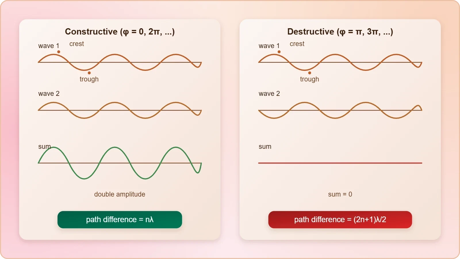
Constructive interference occurs when ##\cos\phi = +1##, that is, when the phase difference is an even multiple of ##\pi## and the path difference is an integral multiple of the wavelength. The resultant amplitude is then the arithmetic sum ##p_{01} + p_{02}##, and for equal amplitudes it doubles, producing a fourfold intensity increase.

Destructive interference occurs when ##\cos\phi = -1##, corresponding to odd multiples of ##\pi## and path differences of odd half-wavelengths. The resultant amplitude becomes ##|p_{01} - p_{02}|##, which vanishes entirely for equal-amplitude sources. The table below consolidates these conditions with their intensity consequences for quick revision.

Intensity Distribution and Energy Conservation

Interference redistributes energy in space without creating or destroying it. At points of constructive interference the intensity exceeds the sum of the individual intensities; at destructive points it falls below. Averaged over a full interference pattern, the total energy equals the sum of the energies the sources would deliver independently, which resolves the apparent paradox of localised energy gain.

For two coherent sources of equal intensity ##I_0##, the resultant intensity at a point with phase difference ##\phi## is ##I = 4I_0\cos^2(\phi/2)##. The average of ##\cos^2(\phi/2)## over all phases is one-half, giving a mean intensity of ##2I_0## — precisely the incoherent sum. Energy conservation is thus satisfied exactly, and the factor of four at maxima is balanced by complete cancellation at minima.

Deriving the intensity relation

Intensity in a sound wave is proportional to the square of the pressure amplitude, ##I \propto p_0^2##. Squaring the resultant amplitude expression from the previous section and applying the half-angle identity converts the amplitude relation into the cosine-squared intensity law. This derivation is short enough to reproduce under exam conditions and is frequently required in JEE Advanced numericals.

For equal intensities this reduces to ##I = 2I_0(1 + \cos\phi) = 4I_0\cos^2(\phi/2)##. The maximum-to-minimum intensity ratio for unequal sources follows directly: ##I_{max}/I_{min} = (p_{01}+p_{02})^2/(p_{01}-p_{02})^2##. A ratio of 25:1, for instance, implies an amplitude ratio of 3:2 between the sources, a standard reverse-engineering question.

Fringe width and spatial pattern

When two coherent point sources separated by distance ##d## radiate into a region, the path difference at a distant point varies with angle ##\theta## from the perpendicular bisector as ##\Delta x = d\sin\theta##. Constructive interference therefore occurs at angles satisfying ##d\sin\theta = n\lambda##, and destructive interference at ##d\sin\theta = (2n+1)\lambda/2##.

The angular separation between adjacent maxima is approximately ##\lambda/d## for small angles, so closer sources or longer wavelengths produce wider fringe spacing. In acoustic demonstrations with two loudspeakers driven at 1 kHz, where ##\lambda \approx 0.34## m, a source separation of 1 m gives maxima roughly every 20 degrees — comfortably audible as alternating loud and quiet zones while walking across a room.

Coherent versus incoherent superposition

Incoherent sources produce no stationary pattern. Their relative phase drifts rapidly compared with the observation time, so the cross term ##2\sqrt{I_1 I_2}\cos\phi## averages to zero and the intensities simply add. Two independent musicians playing the same note illustrate this: the sound is louder but shows no stable spatial structure of reinforcement and cancellation.

Coherent superposition, by contrast, produces a time-independent pattern fixed by geometry. The distinction matters in problem interpretation: questions specifying "two identical sources in phase" imply coherence and demand the full interference treatment, while "two independent sources" signals simple intensity addition. Misreading this cue is a common source of lost marks in JEE Main.

Applying Superposition to JEE Problem Types

Examination questions on superposition cluster into recognisable families: amplitude and intensity calculations from a given phase difference, reverse problems recovering amplitude ratios from intensity ratios, geometric path-difference problems with two sources, and conceptual questions distinguishing coherent from incoherent addition. Each family rewards a fixed procedural approach rather than memorised formulas.

The recommended procedure is consistent. First identify whether the sources are coherent and whether amplitudes are equal. Second, compute the path difference from the stated geometry. Third, convert to phase difference using ##\phi = 2\pi\Delta x/\lambda##. Fourth, apply the amplitude or intensity relation. Fifth, sanity-check the result against the limiting cases of perfect reinforcement and perfect cancellation.

Worked numerical: intensity ratio to amplitude ratio

Suppose two coherent sound sources produce a maximum intensity of 36 units and a minimum of 4 units at different points in space. The amplitude ratio follows from ##I_{max}/I_{min} = 9##, so the amplitude ratio is 3, giving ##(p_{01}+p_{02})/(p_{01}-p_{02}) = 3## and hence ##p_{01}/p_{02} = 2##. The individual intensities stand in the ratio 4:1.

Such reverse problems appear regularly because they test understanding of the squared relationship between amplitude and intensity. A candidate who treats the intensity ratio as an amplitude ratio will obtain 9:1 and lose the mark. The discipline of writing the amplitude relation first, then squaring, prevents this error systematically.

Worked numerical: path difference at a field point

Two in-phase sources separated by 0.5 m emit sound of frequency 680 Hz in air where the speed of sound is 340 m/s. The wavelength is 0.5 m, so the source separation equals exactly one wavelength. A point on the perpendicular bisector has zero path difference and therefore maximum intensity; a point far along the line of the sources has path difference approaching 0.5 m, again a maximum.

At an angle where ##d\sin\theta = \lambda/2##, the path difference is a half-wavelength and the intensity falls to its minimum. With ##d = \lambda##, this occurs at ##\sin\theta = 0.5##, that is, 30 degrees from the perpendicular bisector. The calculation is typical of JEE Main single-correct questions and takes under a minute once the procedure is automatic.

Conceptual traps and exam strategy

Several traps recur. The first is confusing displacement superposition with pressure superposition; for sound, both obey the same linear rule, but the phase relationship between them differs by ##\pi/2##, and questions sometimes exploit this. The second is forgetting that intensity, not amplitude, is what detectors and ears respond to directly.

The third trap concerns the phrase "phase difference of ##\pi##" applied to sources rather than to arrival at a point. An initial phase offset between sources adds directly to the geometric phase difference, so the total is ##\phi_{total} = \phi_{geometric} + \phi_{initial}##. Ignoring the initial offset reverses every constructive and destructive condition in the problem.

Computational check with a short script

A quick numerical script verifies hand calculations and builds intuition for how the intensity pattern varies with phase. The snippet below computes resultant intensity for two equal sources across a range of phase differences and confirms the maximum-to-minimum ratio of four to zero, matching the analytical result.

import numpy as np

I0 = 1.0                      # single-source intensity
phi = np.linspace(0, 2*np.pi, 9)

I_resultant = 4 * I0 * np.cos(phi / 2)**2

for p, I in zip(phi, I_resultant):
    print(f"phi = {p:.3f} rad  ->  I = {I:.3f} I0")

print("Max:", I_resultant.max(), " Min:", round(I_resultant.min(), 6))

Running the script returns a maximum of ##4I_0## at zero phase and a minimum of zero at ##\pi##, with intermediate values following the cosine-squared law. Students preparing for JEE Advanced benefit from reproducing such checks mentally: the pattern's symmetry about ##\pi## and its periodicity of ##2\pi## are structural features that catch sign errors quickly.

From Interference to Standing Waves: Setting Up Lesson 4

The interference machinery developed here applies most powerfully when two waves of equal frequency and amplitude travel in opposite directions. Their superposition produces a standing wave — a pattern with fixed nodes and antinodes rather than travelling maxima. That transition is the subject of Lesson 4, and the intensity relations derived above carry over directly.

Two results from this lesson will be reused immediately. First, the condition for a node is identical to the condition for destructive interference, ##\Delta x = (2n+1)\lambda/2##, now interpreted as a fixed spatial location. Second, the antinode condition matches constructive interference, ##\Delta x = n\lambda##. Recognising this continuity reduces the cognitive load of the next lesson considerably.

Consolidation checklist before proceeding

Before moving to standing waves, verify mastery of five items: the superposition statement and its linearity basis; the amplitude formula for two waves with arbitrary phase; the conversion between path and phase difference; the intensity relation and its energy-conservation interpretation; and the coherent-incoherent distinction. Each is testable in isolation and each feeds directly into the next lesson.

Students who can derive the intensity law from the amplitude expression without reference material, and who can reverse-engineer amplitude ratios from intensity ratios in under two minutes, are prepared for the standing-wave treatment. Those who cannot should revisit the worked numericals above before continuing, because standing-wave problems assume these operations as background.

Applications beyond the syllabus

Interference of sound underlies several technologies worth noting. Active noise cancellation exploits destructive interference by generating an anti-phase wave that cancels unwanted sound, achieving attenuation of 20–30 dB in confined spaces. Acoustic interferometers measure wavelength and speed of sound precisely by tracking the movement of interference maxima as a path length varies.

Medical ultrasound uses constructive interference in phased arrays to steer and focus beams electronically, while architectural acoustics relies on understanding interference to avoid dead spots and uneven coverage in auditoria. These applications share a single analytical core: the superposition of coherent waves and the intensity distribution that results, exactly as derived in this lesson.