Musical Instruments and Harmonics

Musical instruments are, physically speaking, harmonic oscillators engineered to radiate sound efficiently into the surrounding air. A plucked string, a bowed violin, a struck membrane and a blown air column all obey the same underlying wave equation, yet they differ sharply in which frequencies they permit and how strongly each frequency is excited. For the IIT JEE aspirant, this lesson converts the superposition and standing-wave machinery of earlier modules into a quantitative account of pitch, timbre and resonance.

The central analytical claim is that an instrument's harmonic spectrum is fixed by its boundary conditions, while its timbre is governed by the relative amplitudes of those harmonics. A string clamped at both ends supports wavelengths satisfying ##L = n\lambda/2##, whereas a pipe open at both ends and a pipe closed at one end obey different selection rules. These constraints, not the material alone, determine whether a source can produce even harmonics at all.

Building on the shock-wave treatment of Lesson 14, where pressure discontinuities propagate supersonically, this lesson returns to small-amplitude linear acoustics inside resonators. It also prepares the ground for Lesson 15's successor on noise control, where the same spectral reasoning explains why certain harmonics are perceived as harsh and how absorption and damping reduce them.

Fundamental Physics of Musical Sound Production

Every musical instrument performs three coupled functions: it generates a vibration, it selects and amplifies a set of resonant frequencies, and it couples those vibrations to the air as an acoustic radiator. The generator may be a string, an air jet, a reed or a membrane; the resonator may be the instrument body, a tube or a cavity. Separating these roles analytically is the first step toward solving JEE problems on pitch and overtones.

Standing Waves as the Basis of Pitch

A stretched string of length ##L##, tension ##T## and linear mass density ##\mu## carries transverse waves at speed ##v = \sqrt{T/\mu}##. Fixed ends force nodes at both boundaries, so the permitted wavelengths are ##\lambda_n = 2L/n## and the corresponding frequencies follow a simple harmonic series. The fundamental, or first harmonic, sets the perceived pitch.

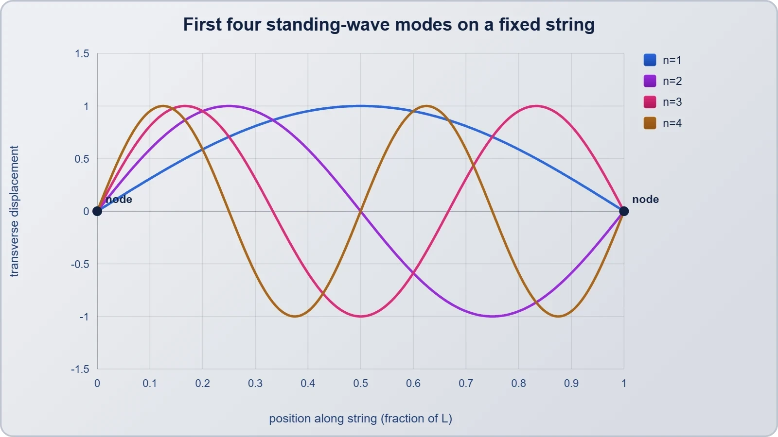
Substituting the wave speed gives the string frequency relation, which JEE candidates should be able to derive from first principles rather than recall:

Three scaling laws follow immediately and appear repeatedly in examination questions. Frequency rises as the square root of tension, falls as the square root of linear density, and falls inversely with length. Doubling the tension raises pitch by a factor of ##\sqrt{2} \approx 1.414##, roughly a tritone, which is why tuning pegs demand fine adjustment.

Air columns obey analogous rules but with different boundary conditions. A pipe open at both ends has pressure nodes at each opening and supports all integer harmonics, while a pipe closed at one end has a pressure antinode at the closed end and admits only odd harmonics. This single distinction explains why clarinets sound hollow compared with flutes.

Open and Closed Pipes: End Correction

Real pipes radiate imperfectly at their openings, so the effective acoustic length exceeds the geometric length by an end correction ##e \approx 0.6r## for a single open end, where ##r## is the tube radius. The corrected fundamental of a closed pipe becomes ##f_1 = v/(4(L + 0.6r))##. This small term explains measurable tuning discrepancies in organ pipes and resonance tubes.

JEE problems frequently test the ratio of fundamental frequencies between an open and a closed pipe of identical length. Ignoring end correction, the closed pipe sounds one octave lower, giving a frequency ratio of 1:2. Including end correction, the ratio shifts slightly, and candidates must decide whether the approximation is justified by the data given.

Resonance tubes in laboratory experiments exploit this relationship directly. A tuning fork of known frequency held over a variable water column produces successive resonances at lengths differing by ##\lambda/2##, allowing the speed of sound to be measured without any timing apparatus. The first resonance occurs near ##\lambda/4##.

Energy, Intensity and Radiation Efficiency

A vibrating string stores energy in both kinetic and elastic forms, and the total energy of the ##n##-th mode scales with the square of its amplitude and frequency. Radiated acoustic intensity depends on the coupling between the vibrating surface and the air, which is poor for a bare string and greatly improved by a soundboard or body.

The radiation efficiency of a source of area ##A## vibrating with velocity amplitude ##u## is captured by the acoustic power relation, where ##\rho## is air density and ##c## the sound speed:

Here ##\sigma## is the radiation efficiency factor, small for dimensions much shorter than the wavelength and approaching unity when the source is comparable to or larger than ##\lambda##. This is why a violin body, not the string, produces most of the audible sound, and why bass instruments require large radiating surfaces.

Damping also matters. A string's vibration decays through internal losses, air drag and energy transfer to the body, and the decay time constant determines sustain. Higher harmonics usually decay faster than the fundamental, so the timbre of a plucked note brightens initially and mellows as it fades.

Harmonic Content and the Character of Instruments

Two instruments playing the same fundamental at the same loudness can sound entirely different because their overtone amplitudes differ. This section treats the harmonic spectrum as a measurable quantity, examines how plucking position and bowing affect it, and connects the analysis to the concept of timbre that JEE questions increasingly probe through superposition arguments.

Fourier Decomposition of a Plucked String

An initial displacement of a string can be expressed as a sum of its normal modes, each with an amplitude determined by the shape of the pluck. A string plucked exactly at its midpoint excites only odd harmonics, because the even modes have a node there and receive zero energy. Plucking nearer the bridge excites a broader spectrum.

The coefficient for the ##n##-th mode of a string plucked at fraction ##\beta## of its length with initial triangular displacement is proportional to ##\sin(n\pi\beta)/n^2##. This compact result predicts that plucking at one-fifth of the length suppresses the fifth harmonic, a fact guitarists exploit to avoid a nasal tone.

import numpy as np

def pluck_spectrum(beta, n_modes=8):
    """Relative amplitudes of harmonics for a string plucked at fraction beta."""
    n = np.arange(1, n_modes + 1)
    amps = np.sin(n * np.pi * beta) / n**2
    return dict(zip(n, np.round(np.abs(amps), 4)))

print(pluck_spectrum(0.5))   # midpoint pluck: even harmonics vanish
print(pluck_spectrum(0.2))   # near-bridge pluck: richer spectrum

Running this decomposition confirms the analytical prediction: at ##\beta = 0.5## the second, fourth and sixth coefficients are numerically zero, while at ##\beta = 0.2## the fifth harmonic vanishes. Such numerical checks build the intuition needed to answer qualitative JEE questions about tone quality quickly.

Bowed strings behave differently because the bow drives the string continuously through a stick-slip mechanism, producing a sawtooth-like waveform rich in harmonics. The harmonic amplitudes fall roughly as ##1/n##, far more slowly than the ##1/n^2## of a plucked string, which is why bowed instruments sound brighter and more sustained.

Wind Instruments: Air Columns and Reed Coupling

In a flute, an air jet directed across the embouchure hole excites the pipe's resonances, and the player selects a register by changing the jet speed and angle. Overblowing at twice the fundamental frequency accesses the second harmonic, which is why flute registers are an octave apart.

Clarinets, being closed-open pipes, overblow at the third harmonic, a twelfth above the fundamental rather than an octave. This structural fact dictates clarinet fingering and explains the instrument's characteristic chalumeau register, where the odd-harmonic dominance produces a dark, hollow timbre distinct from the flute's brighter spectrum.

Reed instruments add a nonlinear coupling between the reed's mechanical vibration and the air column's acoustic pressure. The reed acts as a pressure-controlled valve, and sustained oscillation requires the reed's natural frequency to lie close to a pipe resonance. This phase-locking condition is the acoustic analogue of a driven oscillator near resonance.

Brass instruments extend the same principle with lip vibration as the generator and a flared bell as the radiator. The bell modifies the pipe's resonance frequencies, spreading them so that the natural modes approximate the harmonic series and allow the instrument to play a full chromatic scale with valve additions.

Percussion and Inharmonic Overtones

Percussion instruments depart from the harmonic model because their vibrating elements are two- or three-dimensional. A circular membrane's modes are described by Bessel functions, and the frequency ratios are approximately 1 : 1.59 : 2.14 : 2.30, which are not integer multiples. The result is a sound without a clear pitch.

Timpani solve this problem by loading the membrane with air and enclosing it in a kettle, which shifts the lowest mode and brings the first few overtones closer to harmonic ratios. Xylophone and marimba bars are undercut to tune the first overtone to a specific interval, typically a fourth or an octave above the fundamental.

For JEE purposes, percussion questions usually reduce to standing waves on a bar or membrane with specified boundary conditions. A bar clamped at its centre has an antinode at the centre and nodes near the ends, and its fundamental frequency scales as ##f \propto (t/L^2)\sqrt{Y/\rho}##, where ##t## is thickness and ##Y## Young's modulus.

This scaling explains why shorter, thinner bars sound higher and why marimba makers tune each bar individually by removing material from its underside. The physics is identical to the string case in structure, but the exponent on length differs, a distinction that examiners test deliberately.

Resonance, Beats and Examination Applications

Resonance is the mechanism by which an instrument amplifies a selected frequency, and it is also the source of several classic JEE problem types. This section connects the harmonic analysis of the previous sections to resonance conditions, beat phenomena between nearly tuned sources, and the practical calibration of instruments, while preparing the conceptual ground for the noise-control discussion that follows.

Resonance Conditions and Quality Factor

A driven oscillator responds most strongly when the driving frequency matches a natural frequency, and the sharpness of that response is measured by the quality factor ##Q = f_0/\Delta f##, where ##\Delta f## is the bandwidth at half maximum. High ##Q## means a narrow, sharply tuned resonance.

String instruments exhibit high ##Q##, typically in the hundreds, which gives clean pitch and long sustain. Wind instruments have lower ##Q## because radiation and viscous losses at the walls are larger, so their resonance peaks are broader and the player has more flexibility in pitch through embouchure control.

The amplitude response near resonance follows the standard driven-oscillator form, which JEE candidates should recognise as the same expression derived in the forced-oscillation module:

At resonance ##\omega = \omega_0##, the amplitude reduces to ##F_0/(2m\gamma\omega_0)##, showing that damping alone limits the peak. This is why a heavily damped string, such as one muted by a finger, produces a dull thud rather than a ringing note.

Beats, Tuning and Harmonic Coincidence

When two sources of slightly different frequency sound together, the superposition produces beats at the difference frequency ##f_{beat} = |f_1 - f_2|##. Musicians use this phenomenon to tune instruments, adjusting tension until the beat rate vanishes and the unison is pure.

Beats also arise between harmonics rather than fundamentals. If the second harmonic of one string coincides with the third harmonic of another, the beat frequency is the difference of those harmonic frequencies, which can be much larger than the fundamental beat rate and audibly rougher.

JEE problems often present a tuning fork and a string of unknown frequency, with the beat rate changing when the fork is loaded with wax. The direction of the change reveals whether the string is sharper or flatter than the fork, a standard reasoning step that requires careful sign tracking.

Harmonic coincidence is also the basis of consonance. Intervals whose frequency ratios are simple, such as the octave (2:1) and the perfect fifth (3:2), produce coincident harmonics and are perceived as stable, while complex ratios produce closely spaced but non-coincident harmonics and sound dissonant.

Worked JEE-Style Problem: String and Pipe Combined

Consider a string of length 0.80 m and linear density ##4.0 \times 10^{-3}## kg/m under 64 N tension, sounding alongside a closed pipe of length 0.50 m. The string fundamental is ##f_s = (1/1.6)\sqrt{64/0.004} = 100## Hz, and the pipe fundamental, taking ##v = 340## m/s, is ##f_p = 340/2.0 = 170## Hz.

The beat frequency between these fundamentals is 70 Hz, far too high to hear as beats. However, the third harmonic of the string at 300 Hz and the second harmonic of the pipe at 510 Hz are also non-coincident, so the combination sounds rough rather than beating smoothly, illustrating why harmonic analysis matters.

If the tension is increased until the string's third harmonic coincides with the pipe's second, the required string fundamental becomes 170 Hz, and the tension must rise by the square of the frequency ratio, a factor of ##(170/100)^2 = 2.89##, giving approximately 185 N.

Such problems reward a systematic approach: compute fundamentals, list the permitted harmonics for each resonator type, identify coincidences, then apply the scaling laws. The arithmetic is simple; the difficulty lies in tracking which harmonics each boundary condition allows.

From Harmonics to Noise: A Forward Link

The harmonic framework developed here carries directly into the next lesson on noise control. Noise is, in spectral terms, sound with a dense and inharmonic distribution of energy, and the same resonance and damping arguments explain why absorbers and resonators reduce particular frequency bands.

An instrument's harmonic signature is therefore both a musical asset and, when unwanted, an engineering problem. Understanding which harmonics dominate allows targeted damping, whether in a concert hall, a vehicle cabin or an industrial enclosure, and this continuity is the pedagogical bridge to Lesson 16.

For examination preparation, the essential competencies are: deriving string and pipe frequencies from boundary conditions, predicting harmonic suppression from plucking position, computing beat frequencies between harmonics, and applying scaling laws to tension, length and density. Each is a direct application of superposition and standing waves.

Candidates should also be able to interpret a spectrum qualitatively, distinguishing harmonic from inharmonic content and relating it to perceived pitch and timbre. This interpretive skill increasingly appears in assertion-reason and matching-type questions, where the physics must be stated precisely rather than approximated.