Nonlinear Acoustics and Shock Waves

Linear acoustics treats pressure disturbances as infinitesimal perturbations that travel at a fixed sound speed, and that approximation carries almost every problem in earlier lessons. Real sound waves, however, are finite in amplitude, and once the pressure swing becomes a meaningful fraction of ambient pressure, the medium stops behaving like a perfect linear spring. Compressions heat the gas locally while rarefactions cool it, so the local sound speed varies across a single cycle. That amplitude-dependent speed is the seed from which nonlinear acoustics grows.

This lesson, the twenty-third of thirty in the IIT JEE sound waves sequence, builds directly on acoustic impedance and reflection. Having established how energy partitions at boundaries, we now ask what happens when the wave itself distorts the medium that carries it. The consequences are concrete: waveform steepening, shock formation at finite distances, harmonic generation, and the parametric array, a device that exploits nonlinearity to create highly directional low-frequency beams from compact transducers. Each concept maps onto JEE-relevant reasoning about wave speed, superposition, and energy transport.

Treat the material as a bridge rather than an isolated topic. The steepening mathematics reuses the superposition principle; the shock relations reuse continuity and momentum balance; the parametric array reuses interference. By the end, you should be able to estimate a shock formation distance, explain why a jet crackle differs from a pure tone, and recognise where nonlinear terms enter the wave equation. The next lesson on acoustic filters and mufflers will assume you understand that high-amplitude waves no longer obey simple linear rules.

Origins of Nonlinearity in Finite-Amplitude Sound

Every derivation in linear acoustics assumes the condensation ##s = (\rho - \rho_0)/\rho_0## satisfies ##|s| \ll 1##, which lets us discard second-order terms in the continuity and momentum equations. When the acoustic Mach number ##M = u/c_0## approaches unity, those discarded terms return with measurable force. The medium's response then depends on the instantaneous amplitude, and the wave equation acquires quadratic corrections that linear superposition cannot absorb.

The Thermodynamic Coupling Between Pressure and Sound Speed

For an ideal gas undergoing adiabatic compression, pressure and density follow ##p/\rho^\gamma = \text{constant}##, so the local sound speed scales as ##c = \sqrt{\gamma p/\rho}##. A compression raises both pressure and temperature, increasing ##c## locally; a rarefaction lowers it. The crest of a finite wave therefore outruns the trough, and the waveform skews forward as it propagates. This is the physical engine of all nonlinear acoustic behaviour.

Quantify the effect with the parameter of nonlinearity ##\beta = 1 + B/(2A)##, where ##B/A## is the ratio of second-order to first-order coefficients in the pressure-density expansion. For air, ##\beta \approx 1.2##; for water, ##\beta \approx 3.5##; for biological tissue, values cluster near 4 to 7. A larger ##\beta## means stronger distortion at the same Mach number, which is why medical ultrasound relies on tissue nonlinearity far more than airborne audio does.

The local sound speed can be written as ##c(u) = c_0 + \beta u##, where ##u## is the particle velocity in the direction of propagation. Points of higher forward velocity travel faster, so the wave profile steepens at a rate proportional to ##\beta M##. This single relation explains harmonic generation, shock onset, and the asymmetry between compression and rarefaction phases in one compact statement.

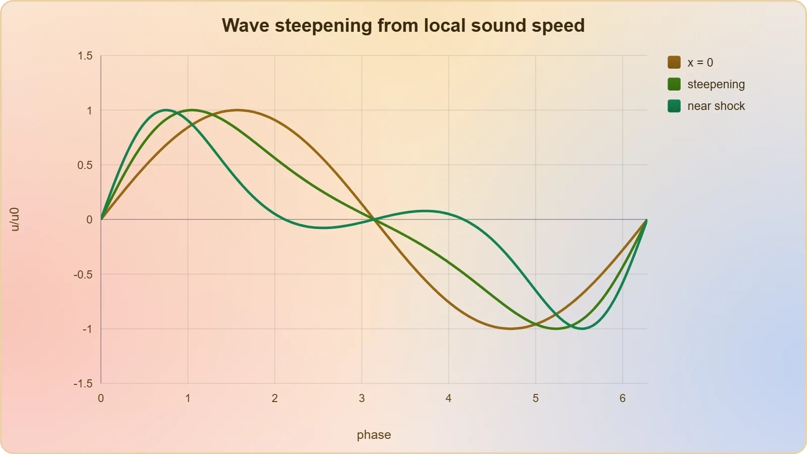
Note the practical threshold. Audible sound at conversational levels has ##M \sim 10^{-7}##, utterly negligible. Jet exhaust noise, explosive blasts, and high-intensity focused ultrasound reach ##M \sim 10^{-2}## to ##10^{-1}##, where nonlinear terms become dominant over distances of metres or centimetres respectively. The transition is gradual, not a switch, and JEE problems typically ask you to identify when the linear approximation fails.

Deriving the Nonlinear Wave Equation

Start from the one-dimensional continuity equation ##\partial_t \rho + \partial_x(\rho u) = 0## and the momentum equation ##\rho(\partial_t u + u \partial_x u) = -\partial_x p##, retaining all convective terms. Expand pressure as ##p = p_0 + A s + \tfrac{1}{2} B s^2## and substitute. The quadratic terms survive, producing a wave equation with a source term proportional to ##\partial_x(u^2)## rather than a clean linear operator.

A cleaner route uses the method of characteristics. Define the Riemann invariants ##J_\pm = u \pm \int dp/(\rho c)##; in a lossless medium these propagate unchanged along characteristics with slopes ##u \pm c##. Because the slope depends on ##u##, characteristics of the same family converge where the wave is compressive. Their intersection marks the birth of a discontinuity, and the distance to that intersection is the shock formation distance.

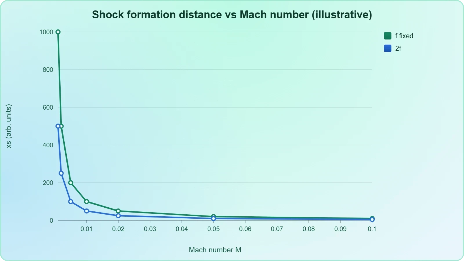
For a sinusoidal source of angular frequency ##\omega## and initial amplitude ##u_0##, the formation distance is:

where ##k = \omega/c_0## is the wavenumber and ##M = u_0/c_0## the acoustic Mach number. The inverse dependence on both frequency and amplitude is the key examinable result: doubling either halves the distance over which a clean sine becomes a sawtooth. In air at 1 kHz with ##u_0 = 10\ \text{m/s}##, ##x_s## is roughly 4 metres, which is why loud brass instruments crackle within a concert hall.

Harmonic Generation and Energy Transfer

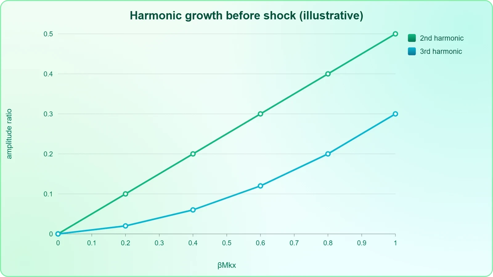
Before the shock forms, the distortion appears as harmonics. A pure sine at frequency ##f## develops components at ##2f##, ##3f##, and beyond, with the second-harmonic amplitude growing as ##\propto \beta M k x## for small distances. Energy migrates steadily from the fundamental into higher harmonics, thinning the fundamental and enriching the spectrum. This is why nonlinear propagation audibly brightens a loud tone.

The harmonic cascade is not free. Each harmonic experiences stronger absorption than its parent because attenuation scales roughly as ##f^2## in most fluids, so the medium eventually dissipates the transferred energy as heat. The competition between nonlinear energy transfer toward high frequencies and viscous-thermal absorption at high frequencies produces the characteristic "shock" spectrum with its broad, slowly decaying tail.

For JEE purposes, treat harmonic generation qualitatively but quantitatively where asked. If a problem states that the second harmonic reaches 10% of the fundamental after 2 metres, you can infer the product ##\beta M k## and predict behaviour at other distances. Recognise that linear superposition of two tones fails here: the sum of two sines no longer propagates as the sum of two independently evolving sines.

One subtlety deserves emphasis. The nonlinearity is a property of the medium, not the source. A transducer emitting a perfect sinusoid still produces harmonics after sufficient propagation, because the medium itself manufactures them. Conversely, a distorted source waveform in a very low-amplitude field will linearise as it propagates, since the nonlinear terms become negligible relative to the linear ones.

Shock Waves: Formation, Structure, and Jump Conditions

Once characteristics intersect, the mathematical solution becomes multivalued, which is physically impossible. Nature resolves this by inserting a thin discontinuity, the shock front, across which pressure, density, temperature, and velocity jump abruptly. The front is not infinitely sharp; viscosity and thermal conduction smear it over a few mean free paths, but for engineering purposes it behaves as a surface.

The Rankine–Hugoniot Relations

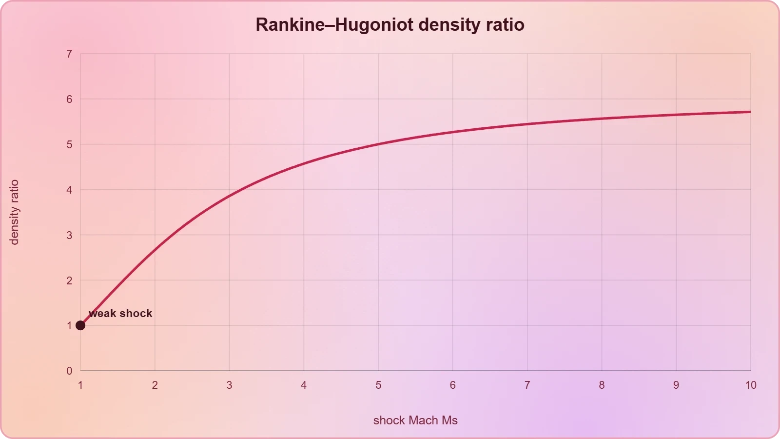
Apply conservation laws across the shock in the frame moving with the front. Mass, momentum, and energy conservation give three algebraic relations linking upstream state 1 to downstream state 2. For a perfect gas with specific heat ratio ##\gamma##, the pressure ratio follows the Hugoniot relation:

where ##M_s## is the shock Mach number relative to the upstream sound speed. For weak shocks with ##M_s \to 1##, this reduces to the acoustic result ##\Delta p = \rho_0 c_0 \Delta u##, confirming continuity with linear theory. For strong shocks, the pressure ratio grows without bound while the density ratio saturates at ##(\gamma+1)/(\gamma-1)##, equal to 6 for air.

That density saturation is a striking result. However hard you drive a shock into air, the downstream density cannot exceed six times the upstream value, because the excess energy goes into heating rather than compression. Temperature, by contrast, rises without limit, which is why re-entry vehicles and hypersonic projectiles face severe thermal loads even at moderate density ratios.

Entropy increases across the shock, so the process is irreversible. This irreversibility is the source of the familiar sonic boom's energy loss and the crack of a whip, where the tip briefly exceeds the local sound speed and radiates a small shock. The Rankine–Hugoniot relations are the acoustic analogue of a hydraulic jump, and the mathematics transfers directly.

Weak Shock Theory and the Sawtooth Wave

For weak shocks, the full Rankine–Hugoniot machinery simplifies considerably. The waveform evolves toward a sawtooth profile whose leading edge is a near-discontinuity and whose trailing edge is a gradual ramp. The amplitude decays as ##1/\sqrt{x}## in a lossless medium, slower than the exponential decay of a linear pulse, because the shock continuously feeds energy forward.

This algebraic decay law is a favourite examination point. It explains why a distant explosion still delivers a sharp report while a linear pulse of the same initial energy would have smeared into inaudibility. The sawtooth's asymmetry, with a steep compression front and a slow rarefaction tail, also explains the directional character of blast noise.

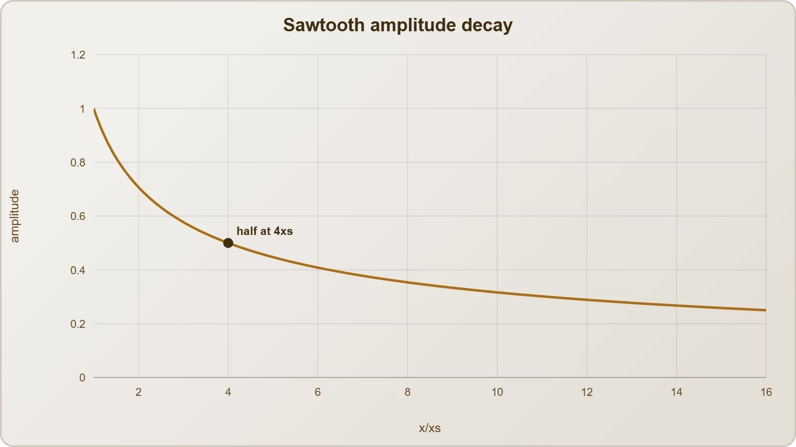
Practical shock formation distances in air span a wide range. A firecracker at 1 metre produces a shock within centimetres; a supersonic aircraft's sonic boom forms at the aircraft and propagates as a Mach cone, reaching the ground as an N-wave with a characteristic double bang. The N-wave shape, with abrupt pressure rises at both ends, is the far-field signature of a finite-amplitude pulse.

For problem-solving, remember the scaling chain: ##x_s \propto 1/(\beta M k)##, post-shock amplitude ##\propto x^{-1/2}##, and shock thickness ##\propto 1/M_s## for weak shocks. These three relations cover most JEE-style questions on the topic, and each follows from the conservation laws rather than from memorisation.

Dissipation, Dispersion, and the Burgers Equation

Balancing nonlinear steepening against viscous diffusion yields the Burgers equation, ##\partial_t u + u \partial_x u = \nu \partial_{xx} u##, the simplest model retaining both effects. Its steady travelling-wave solutions are the weak shock profiles, and its Reynolds number ##Re = u_0/(\nu k)## determines whether steepening or diffusion dominates. High ##Re## gives sharp shocks; low ##Re## gives smooth, nearly linear waves.

The Burgers equation is a workhorse because it admits exact solutions via the Cole–Hopf transformation, converting the nonlinear problem into a linear diffusion equation. For JEE aspirants, the value lies in recognising the structure: a convective term that steepens and a diffusive term that smooths. The same competition appears in traffic flow and in nonlinear optics.

Dispersion adds a third ingredient. In media where sound speed varies with frequency, such as bubbly liquids or the ionosphere, dispersive spreading can counteract nonlinear steepening and produce stable solitary waves rather than shocks. These solitons preserve their shape through collisions, a phenomenon that linear superposition cannot produce and that marks a clean departure from the earlier lessons.

Keep the regimes distinct in your mind. Pure nonlinearity gives shocks; nonlinearity plus diffusion gives smooth shock profiles; nonlinearity plus dispersion gives solitons. Each regime has its own governing equation and its own characteristic length scale, and identifying which regime a problem inhabits is often the hardest step.

Parametric Arrays and Practical Nonlinear Acoustics

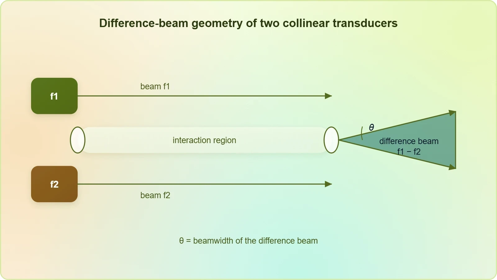
The parametric array exploits nonlinearity deliberately. Two intense, collinear, high-frequency beams at frequencies ##f_1## and ##f_2## interact within the medium to generate difference-frequency sound at ##f_1 - f_2##. Because the difference-frequency source is distributed along the beam rather than located at a physical aperture, the resulting low-frequency beam is extraordinarily narrow, often a few degrees wide.

Operating Principle of the Parametric Array

The interaction region is confined to the overlap of the two primary beams, which is itself narrow because high frequencies are highly directional. The generated difference-frequency source therefore has the shape of a long, thin cylinder, and its far-field directivity is set by that virtual aperture. The effective aperture length is limited by absorption of the primaries, typically a few metres in water.

Efficiency is low, often below one percent, because most primary energy is absorbed rather than converted. The trade-off is worthwhile where directivity matters more than efficiency: underwater communication, sonar, and audio spotlights that project sound into a confined zone. The audio spotlight is the most familiar consumer application, using ultrasound primaries in air to create a beam of audible sound.

The mathematics of the difference-frequency generation follows from the quadratic nonlinear term. The source strength is proportional to ##\beta##, the product of primary amplitudes, and a phase-matching factor that is automatically satisfied for collinear beams in a nondispersive medium. The generated pressure grows linearly with interaction length until absorption of the primaries truncates the process.

For JEE-level analysis, the key relations are the difference frequency ##f_- = |f_1 - f_2|##, the narrow beamwidth scaling ##\theta \propto \lambda_-/L_{\text{eff}}##, and the quadratic dependence of generated amplitude on primary amplitude. These three facts explain why parametric arrays need high-intensity primaries and why they produce such tightly confined low-frequency beams.

Applications from Medical Ultrasound to Jet Noise

Medical imaging uses tissue nonlinearity to improve resolution. Tissue harmonic imaging transmits at one frequency and receives at twice that frequency, exploiting the cleaner propagation of the harmonic to reduce clutter from body wall echoes. The technique is now standard on most clinical scanners and relies directly on the harmonic generation described earlier.

High-intensity focused ultrasound uses nonlinear focusing to concentrate energy at a target for ablation, with shock formation enhancing the local heating rate. Lithotripsy, the breaking of kidney stones, depends on shock waves generated outside the body and focused to a point. Both applications turn the shock-formation distance into a design parameter rather than a nuisance.

Jet noise is the engineering counterexample. The turbulent mixing layer of a high-speed jet radiates sound whose peak amplitude is high enough to form weak shocks, producing the characteristic crackle of military aircraft. Suppressing crackle requires reducing either the Mach number or the coherence of the turbulent structures, which is why chevron nozzles and lobed mixers appear on modern engines.

Industrial and environmental acoustics also feel nonlinearity. Sonic booms from supersonic flight, blast waves from explosions, and the roar of rocket launches all involve finite-amplitude propagation over kilometres. Predicting their ground-level signatures requires the full nonlinear machinery, and the regulatory limits on supersonic overland flight are written in terms of the resulting shock overpressure.

Worked Problem: Estimating Shock Formation in Air

Consider a loudspeaker radiating a 2 kHz tone with particle velocity amplitude ##u_0 = 5\ \text{m/s}## into air at ##c_0 = 343\ \text{m/s}## and ##\beta = 1.2##. Compute the shock formation distance and comment on whether the linear approximation holds over a typical room. This is a representative JEE-style estimation problem combining wave speed, nonlinearity, and order-of-magnitude reasoning.

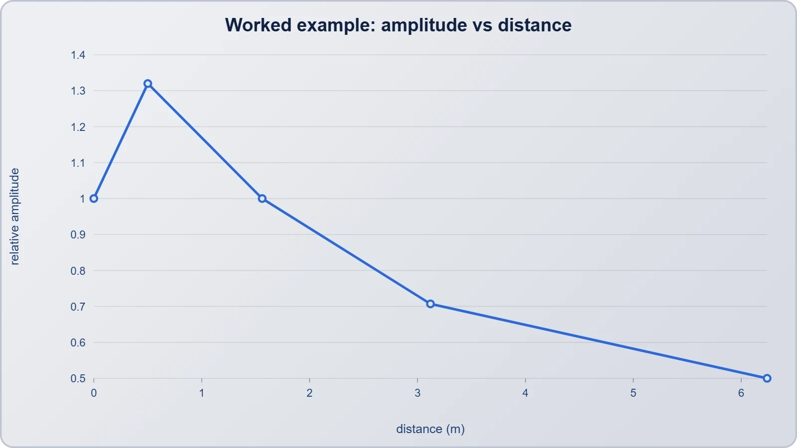
First compute the Mach number: ##M = 5/343 \approx 0.0146##. The wavenumber is ##k = 2\pi f/c_0 = 2\pi(2000)/343 \approx 36.6\ \text{rad/m}##. Then ##x_s = 1/(\beta M k) = 1/(1.2 \times 0.0146 \times 36.6) \approx 1.56\ \text{m}##. The shock forms within about 1.6 metres, well inside a room, so linear theory fails at realistic listening distances.

Now check the harmonic growth before the shock. At 0.5 metres, the second-harmonic amplitude relative to the fundamental is roughly ##\beta M k x /2 \approx 0.32##, or 32%. That is a substantial spectral change, audible as added brightness. The linear approximation is already poor at half a metre, long before the shock itself forms.

Finally, consider the post-shock decay. Beyond 1.56 metres, the sawtooth amplitude falls as ##x^{-1/2}##, so at 6.24 metres (four times the formation distance) the amplitude is half its value at formation. This algebraic decay is far slower than the exponential decay a linear pulse would suffer, explaining why loud high-frequency tones remain audible across large halls.

Connecting Forward: From Nonlinearity to Acoustic Filters

This lesson closes the loop between the linear wave theory of earlier lessons and the engineering devices of the next. Acoustic filters and mufflers are designed on linear assumptions, but their performance degrades when the incident sound is intense enough to trigger nonlinear effects. A muffler tuned for a linear impedance mismatch may leak harmonics generated upstream.

Carry forward three durable ideas. First, nonlinearity is a medium property quantified by ##\beta##, and it becomes significant when ##\beta M k x## approaches unity. Second, shocks are the inevitable endpoint of finite-amplitude compression, governed by Rankine–Hugoniot jump conditions and decaying algebraically. Third, the parametric array shows that nonlinearity can be engineered into a useful tool rather than merely tolerated.

For examination preparation, practise the scaling relations until they are automatic: formation distance, harmonic growth, post-shock decay, and the weak-shock limit recovering linear acoustics. Each is a short derivation from conservation laws, and each appears in JEE-style problems framed around loudspeakers, explosions, or medical devices. Mastery here means recognising which regime applies before reaching for a formula.

The next lesson on acoustic filters and mufflers returns to linear territory but with a sharper appreciation of its limits. You will design reactive and dissipative elements using impedance and transmission-line reasoning, and you will now know when those designs must be qualified by nonlinear caveats. That awareness distinguishes a competent solver from a merely formula-driven one.