Standing Waves in Strings and Pipes

Standing waves represent the most consequential outcome of the superposition principle covered in the preceding lesson: when a wave reflects at a boundary and interferes with its own incident counterpart, energy ceases to travel and instead settles into fixed spatial nodes and antinodes. For IIT JEE aspirants, this transition from travelling to stationary disturbance is where qualitative wave theory becomes quantitative problem-solving. The examination routinely tests string harmonics, organ pipe resonances, end corrections, and the subtle distinction between overtone numbering in open and closed columns.

This fourth lesson of thirty builds directly on interference and prepares the ground for resonance and forced vibrations. The treatment is deliberately structural: boundary conditions determine which wavelengths survive, and every formula follows from those conditions rather than from memorisation. Strings fixed at both ends, pipes open at both ends, and pipes closed at one end each admit a distinct harmonic series, and the differences between them carry heavy examination weight. Worked derivations, comparative tables, and JEE-pattern calculations anchor each concept.

Two governing relations recur throughout. The wave speed on a stretched string obeys ##v=\sqrt{T/\mu}##, where ##T## is tension and ##\mu## the linear mass density, while the speed of sound in a gas column follows ##v=\sqrt{\gamma RT/M}##. Every standing-wave frequency is then obtained by inserting the permitted wavelengths into ##f=v/\lambda##. Mastery lies in identifying the boundary conditions first, deriving the allowed wavelengths second, and only then substituting numerical values.

Formation of Standing Waves: Boundary Conditions and Node Structure

A standing wave forms when two identical waves of equal amplitude travel in opposite directions through the same medium. Reflection at a rigid or free boundary generates the counter-propagating component, and the resulting displacement pattern is described by ##y=2A\sin(kx)\cos(\omega t)##. The spatial envelope ##2A\sin(kx)## is fixed in place, oscillating in time but never translating, which is precisely why the configuration is termed stationary.

Reflection at Rigid and Free Boundaries

At a rigid boundary, such as a string clamped to a wall, the reflected wave undergoes a phase inversion of ##\pi## radians. The incident and reflected displacements therefore cancel at the boundary, forcing a displacement node there. This single condition, that displacement must vanish at a fixed end, constrains every permitted wavelength on the string and ultimately generates the entire harmonic series.

At a free boundary, exemplified by the open end of an air column, the reflected wave returns without phase inversion. Displacement reaches a maximum at that point, producing an antinode, while pressure conversely reaches a node because the open end communicates with the constant atmospheric pressure outside. This displacement-pressure inversion at open ends is a frequent source of examination error and deserves explicit attention.

The distance between adjacent nodes is always ##\lambda/2##, and between a node and the nearest antinode exactly ##\lambda/4##. These spacings are independent of the medium, the frequency, or the boundary type, making them reliable anchors when reconstructing a wavelength from a described pattern. JEE questions frequently supply node positions and demand the harmonic number, which these spacings resolve directly.

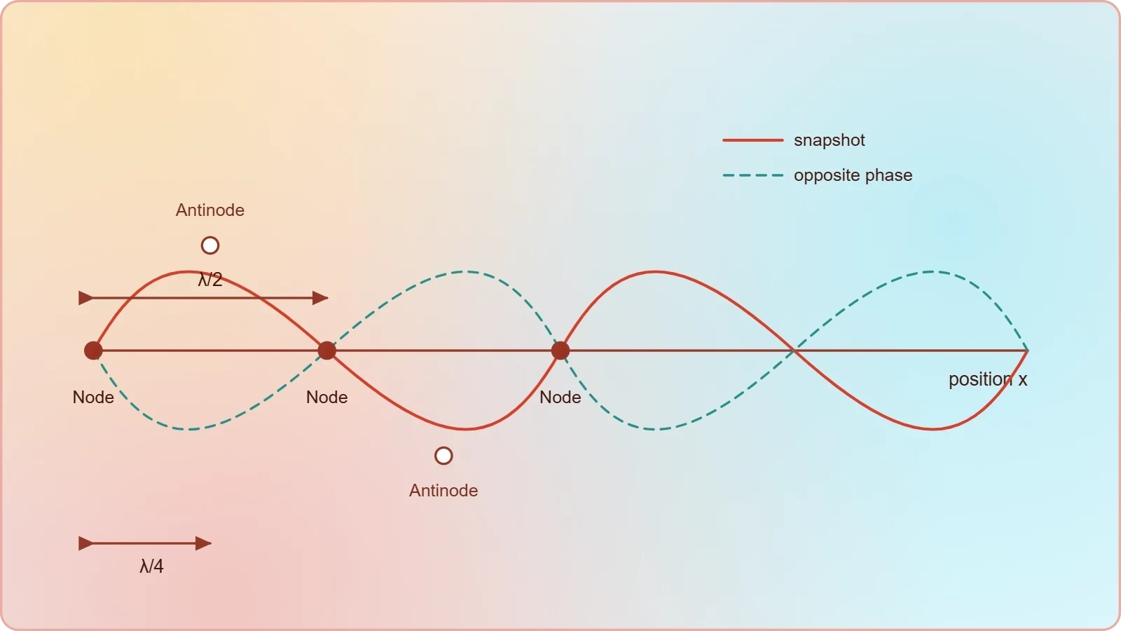
Energy considerations complete the physical picture. A travelling wave transports energy continuously along the medium, whereas a standing wave confines energy within segments, oscillating between purely kinetic and purely elastic forms twice per cycle. The nodes remain permanently at rest, and no net energy crosses them, which explains why a plucked string radiates sound only through its coupling to the surrounding air.

Nodes, Antinodes, and Energy Localisation

Nodes are points of permanently zero displacement, while antinodes oscillate with maximum amplitude ##2A##. Between consecutive nodes the medium moves in phase, and adjacent segments oscillate in antiphase with one another. This alternating phase structure is visible in Melde-type demonstrations and explains why a vibrating string appears to divide into discrete loops rather than a continuous blur.

Because no energy crosses a node, each loop behaves as an isolated oscillator exchanging energy internally. The total energy of the standing wave equals the sum of the energies of the two constituent travelling waves, but it remains spatially trapped. This localisation underpins the resonance behaviour examined in the next lesson, where external driving at a natural frequency pumps energy into these confined modes.

Mathematical Description of the Stationary Pattern

Applying the boundary condition ##y(0,t)=0## to the general solution forces ##\sin(k\cdot 0)=0##, which is automatically satisfied, while the second boundary at ##x=L## demands ##\sin(kL)=0##. Hence ##kL=n\pi## for integer ##n##, giving the quantisation condition ##L=n\lambda/2##. The allowed wavelengths are therefore discrete, and no intermediate wavelength can sustain a standing wave on a fixed-fixed string.

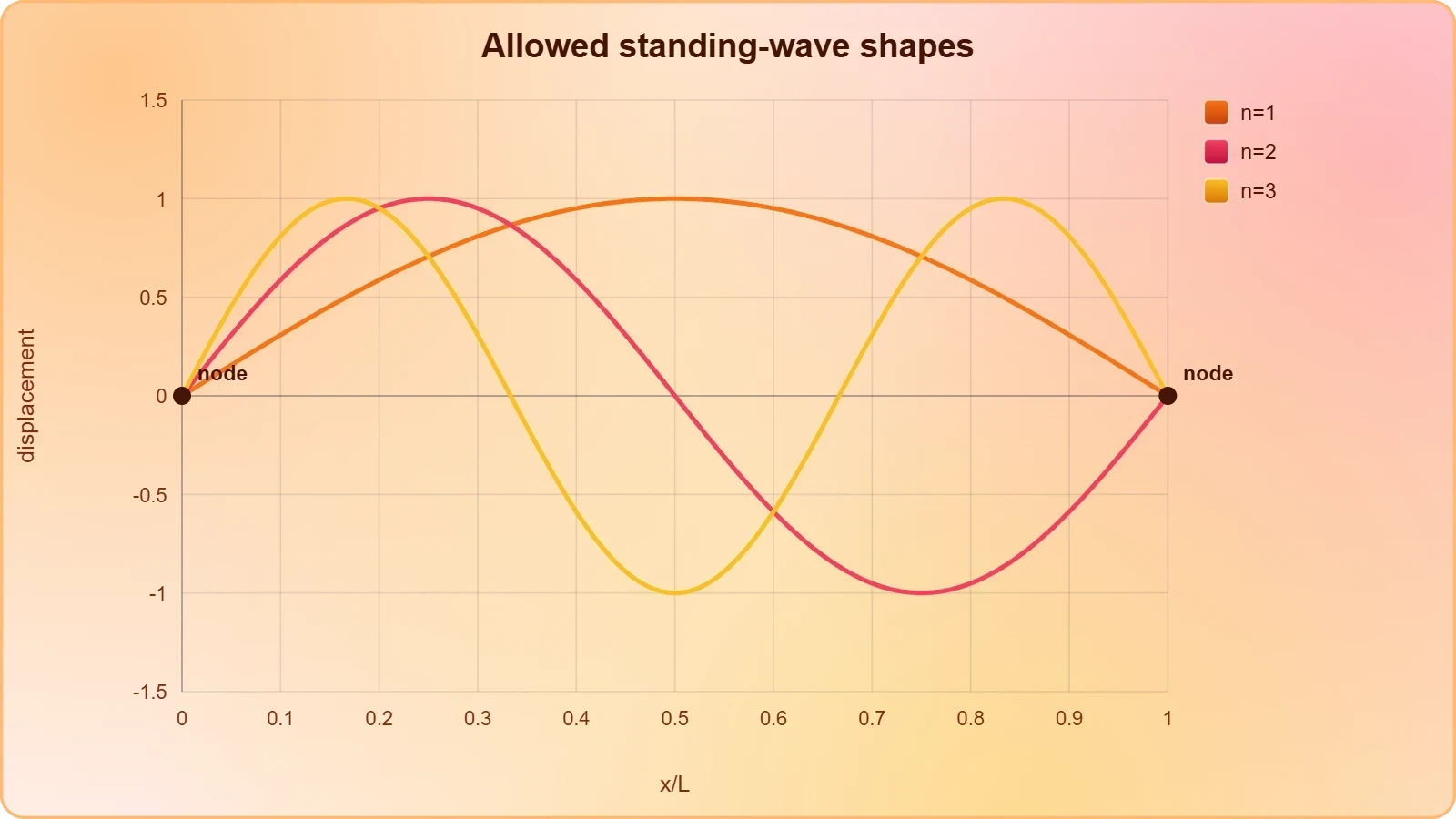
This quantisation is mathematically identical to the condition for allowed electron orbits in a Bohr atom, a correspondence worth noting for conceptual economy. In both cases a wave must close on itself consistently after one round trip, and destructive self-interference eliminates every other configuration. The integer ##n## counts the number of half-wavelengths fitting within the length ##L##.

Worked Example: Reconstructing a Pattern from Data

Consider a string of length ##1.2\ \text{m}## vibrating in its third harmonic. The condition ##L=3\lambda/2## yields ##\lambda=0.8\ \text{m}##, and with a wave speed of ##240\ \text{m/s}## the frequency follows as ##f=v/\lambda=300\ \text{Hz}##. The string contains three loops, four nodes including both ends, and three antinodes at positions ##0.2##, ##0.6##, and ##1.0\ \text{m}##.

import math

def string_harmonic(L, n, tension, mu):
    # Fixed-fixed string: L = n * lambda / 2
    lam = 2 * L / n
    v = math.sqrt(tension / mu)
    f = v / lam
    return lam, v, f

lam, v, f = string_harmonic(L=1.2, n=3, tension=96.0, mu=0.0016)
print(f"Wavelength = {lam:.3f} m, Speed = {v:.1f} m/s, Frequency = {f:.1f} Hz")

Harmonics and Overtones in Stretched Strings

A string fixed at both ends supports all integer multiples of its fundamental frequency, forming a complete harmonic series. The fundamental, or first harmonic, corresponds to ##n=1## with a single loop and wavelength ##2L##. Successive harmonics add one loop each, and the ##n##-th harmonic has frequency ##f_n=nf_1##, where ##f_1=\dfrac{1}{2L}\sqrt{T/\mu}##.

The Fundamental Frequency and Its Dependence on Parameters

The fundamental frequency scales as the square root of tension and inversely as the square root of linear density. Doubling the tension raises the pitch by a factor of ##\sqrt{2}\approx1.414##, a result exploited by musicians tuning stringed instruments. Halving the vibrating length doubles the frequency, which is why a guitarist shortens the string by pressing a fret.

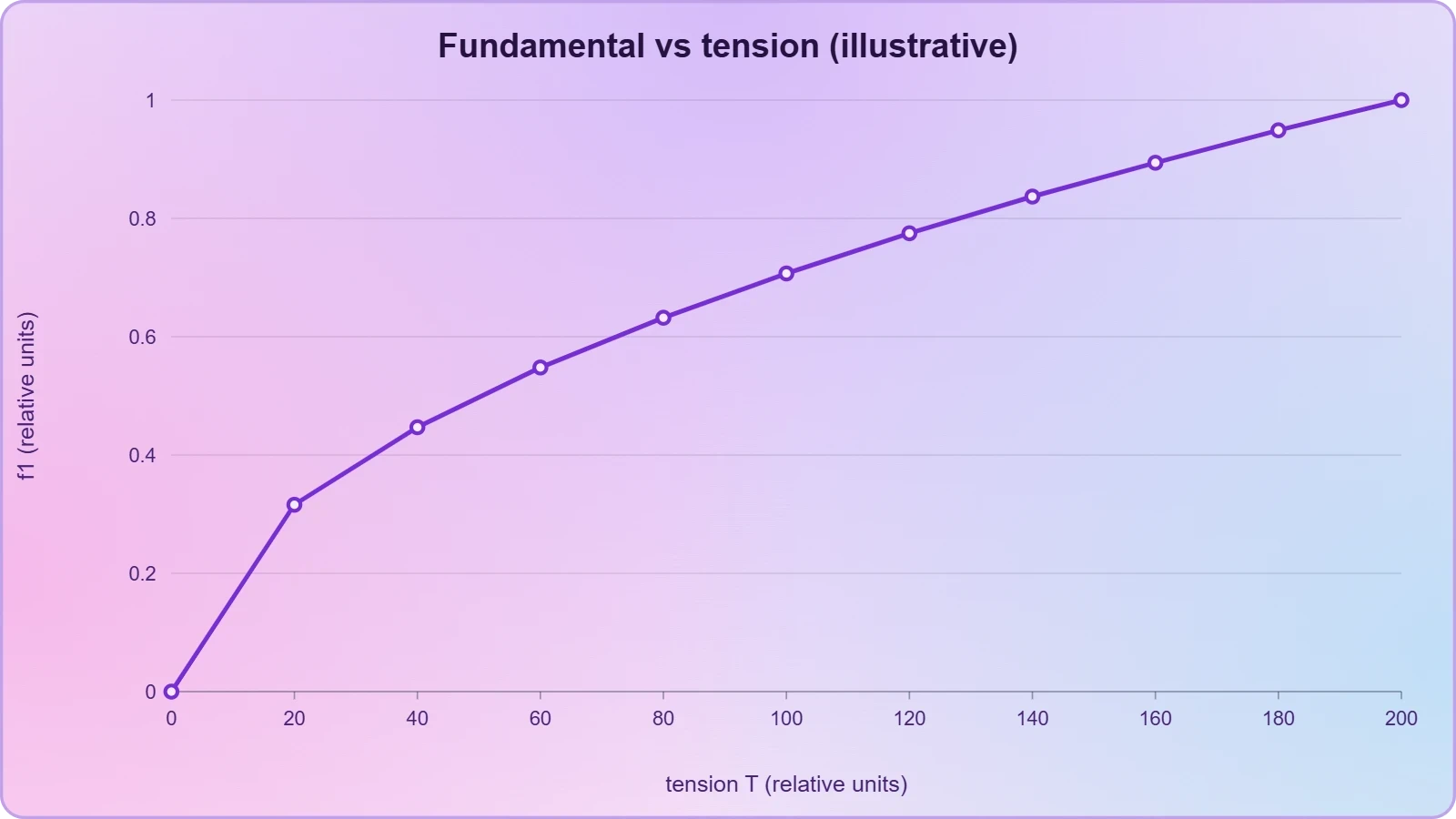
Linear density depends on the material and cross-sectional area, so a thicker string of identical material and tension sounds lower. Steel strings therefore require greater tension than nylon strings of comparable gauge to reach the same pitch. JEE problems frequently combine these dependencies, asking how frequency changes when tension, length, and radius are altered simultaneously.

Overtones and the Harmonic Series

For a fixed-fixed string, the overtone numbering coincides with the harmonic numbering offset by one: the first overtone is the second harmonic, the second overtone the third harmonic, and so on. This coincidence holds only for systems supporting the complete integer series, and it breaks down entirely for pipes closed at one end, where only odd harmonics appear.

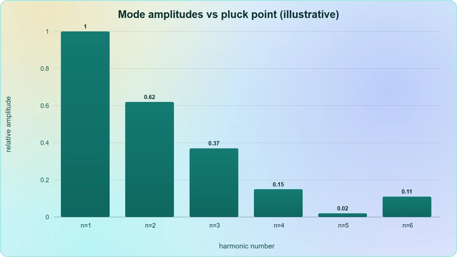
The presence of all harmonics gives a plucked string its rich timbre, since the initial triangular displacement decomposes into a Fourier superposition of many modes. The relative amplitudes of these modes depend on where the string is plucked; plucking at the midpoint suppresses all even harmonics because that point is a node for every even mode. This is a favourite conceptual question in JEE Advanced.

JEE-Pattern Problem: Combined Parameter Change

Suppose a string's tension increases by ##21\%## while its length is reduced by ##10\%##. The frequency ratio becomes ##\sqrt{1.21}/0.9=1.1/0.9\approx1.222##, a net increase of roughly ##22.2\%##. Such problems reward careful separation of the square-root dependence on tension from the inverse-linear dependence on length, and they appear with predictable regularity.

Nodes as Measurement Anchors

Because node positions are fixed and measurable, they provide a practical route to wavelength determination in laboratory settings. Measuring the distance between three consecutive nodes gives one full wavelength directly, avoiding the need to locate antinodes, which are harder to pinpoint precisely. Sonometers exploit exactly this principle when determining the frequency of a tuning fork.

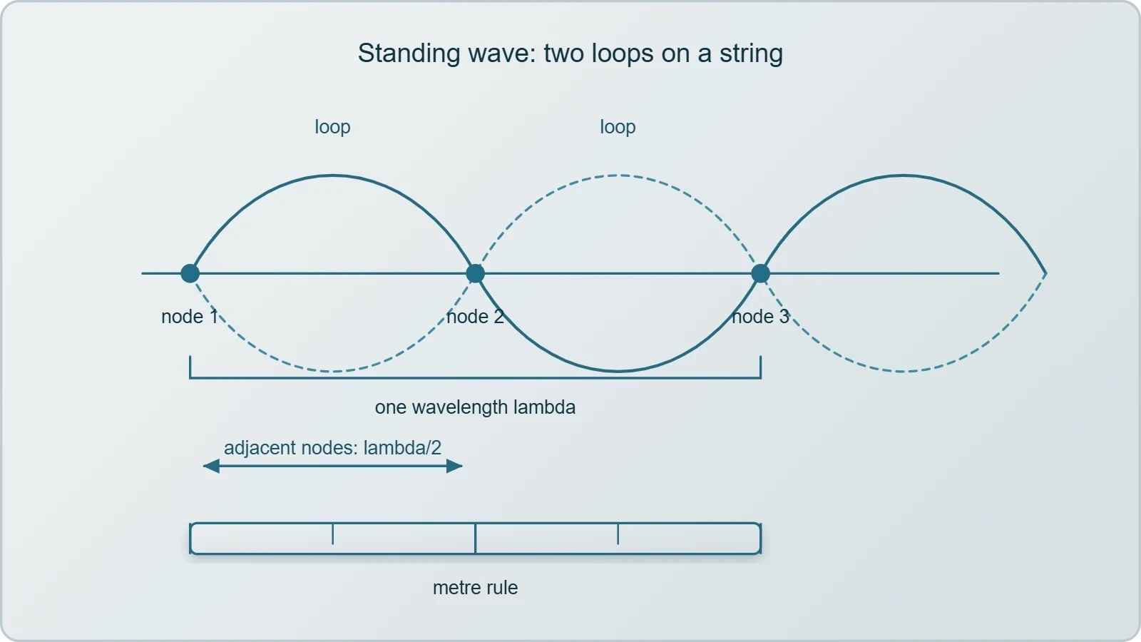
In a sonometer experiment, the vibrating string's fundamental is matched against a known fork, and the resonance condition ##f=\dfrac{1}{2L}\sqrt{T/\mu}## then permits calculation of any unknown among tension, length, or density. The precision of the method depends on node sharpness, which improves with higher tension and thinner strings. Typical school experiments achieve agreement within two or three percent.

Limits of the Ideal String Model

Real strings possess bending stiffness, so the ideal wave equation holds only approximately, and inharmonicity appears in stiff strings such as piano wire. The frequencies then deviate slightly from exact integer multiples, producing the characteristic stretched tuning of pianos. JEE problems ignore this correction, but recognising its existence prevents overgeneralisation of the ideal model.

Damping also broadens each resonance and causes the amplitude to decay over time, converting the ideal infinite-Q oscillator into a finite-bandwidth resonator. The quality factor ##Q=f_0/\Delta f## quantifies this sharpness and connects directly to the forced-oscillation treatment in the following lesson. For examination purposes, undamped ideal strings remain the operative assumption.

Standing Waves in Open and Closed Air Columns

Air columns support longitudinal standing waves whose boundary conditions differ fundamentally from those of strings. At an open end the air is free to move, producing a displacement antinode and a pressure node, whereas a closed end constrains displacement to zero and generates a pressure antinode. These complementary conditions produce two distinct harmonic families with markedly different frequency spectra.

Pipes Open at Both Ends

A pipe open at both ends possesses antinodes at each extremity and therefore supports all integer harmonics, exactly like a fixed-fixed string. The condition ##L=n\lambda/2## yields fundamental frequency ##f_1=v/2L##, and the ##n##-th harmonic is ##nf_1##. The full harmonic series gives open pipes a timbre comparable to that of strings.

Because both ends are open, the air column behaves symmetrically, and the pressure distribution is the mirror image of the displacement distribution. Pressure nodes occur at the open ends and pressure antinodes at the midpoint for the fundamental. Questions often ask for the pressure pattern rather than the displacement pattern, and the two must be carefully distinguished.

Pipes Closed at One End

A pipe closed at one end and open at the other supports only odd harmonics, because the boundary conditions require a node at the closed end and an antinode at the open end. The permitted lengths satisfy ##L=(2n-1)\lambda/4##, giving frequencies ##f=(2n-1)v/4L##. The fundamental is ##v/4L##, exactly half that of an open pipe of identical length.

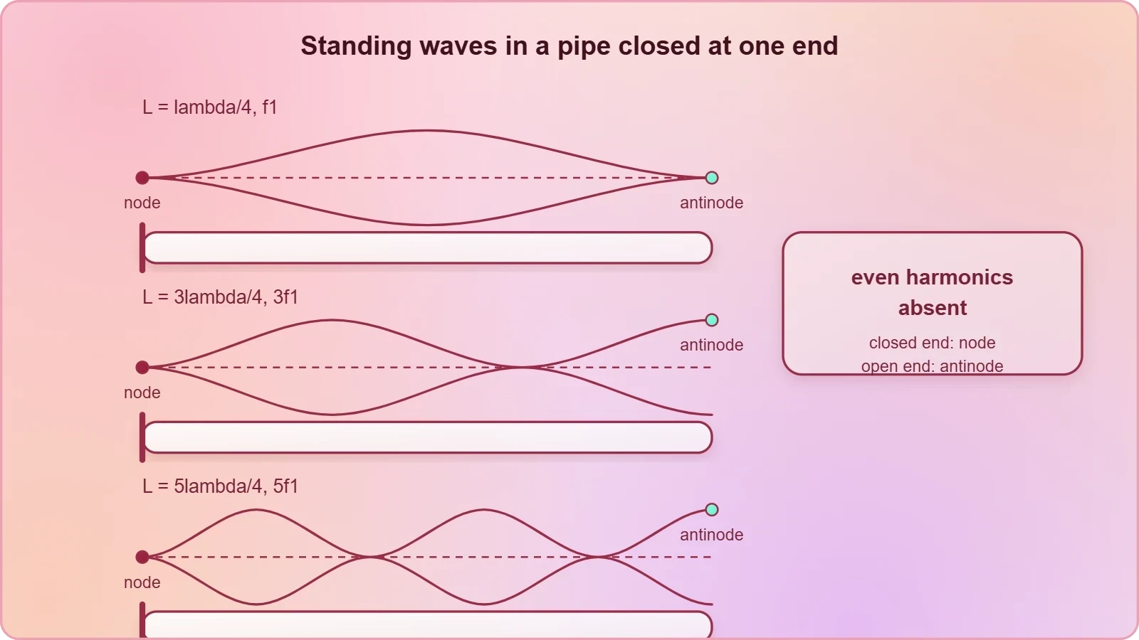
This halving means a closed pipe sounds one octave below an open pipe of the same length, a fact with direct musical consequences in organ design. The absent even harmonics give closed pipes a hollow, clarinet-like quality, whereas open pipes sound brighter. The first three allowed frequencies stand in the ratio ##1:3:5##, a ratio worth committing to memory.

Overtone numbering in closed pipes is a notorious trap. The first overtone is the third harmonic, the second overtone the fifth harmonic, and the ##k##-th overtone corresponds to harmonic ##2k+1##. Candidates who mechanically apply the string convention lose marks, so the odd-only rule should be verified against the boundary conditions every time.

End Correction and Real Pipe Behaviour

The displacement antinode at an open end actually lies slightly outside the physical pipe, because the surrounding air participates in the motion. The effective length therefore exceeds the geometric length by approximately ##0.6r## at each open end, where ##r## is the pipe radius. This end correction shifts all resonant frequencies downward and matters in precise measurements.

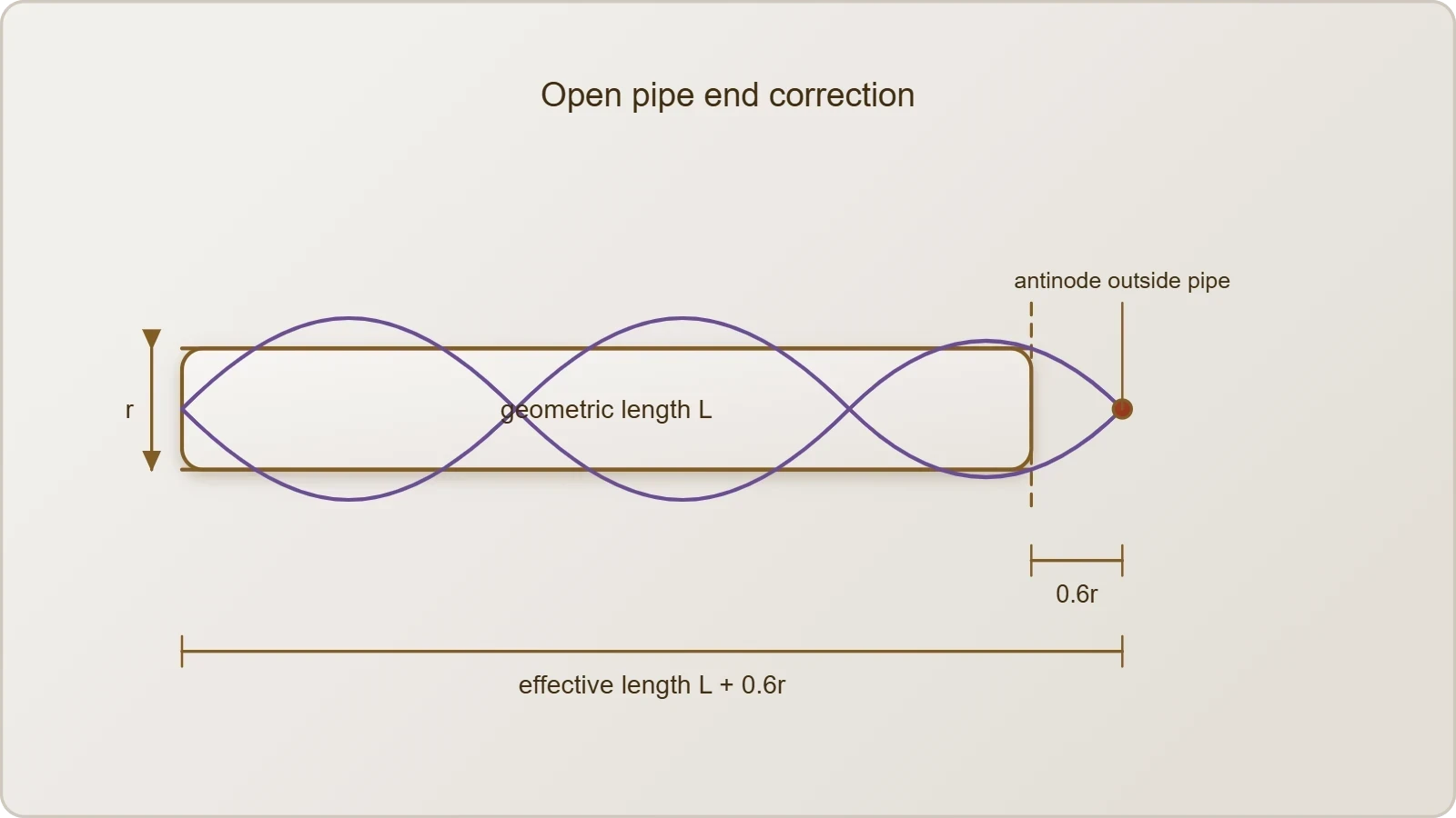
For a pipe open at both ends, the corrected fundamental becomes ##f_1=v/[2(L+1.2r)]##, while for a closed pipe the correction applies only at the single open end. JEE problems occasionally supply two resonance lengths and require the end correction to be eliminated, a standard technique worth rehearsing. The difference between successive resonance lengths isolates the correction neatly.

Temperature also alters pipe resonance, since ##v\propto\sqrt{T}## in kelvin. A rise from ##27^\circ\text{C}## to ##47^\circ\text{C}## raises the speed by roughly ##3.3\%##, shifting every resonant frequency upward by the same fraction. Organ builders compensate for this drift, and examination questions sometimes embed it within a combined gas-law and wave-speed calculation.

Worked Example: Two Resonance Lengths

A tuning fork produces resonance in a closed pipe at lengths of ##0.17\ \text{m}## and ##0.51\ \text{m}##. The difference ##0.34\ \text{m}## equals ##\lambda/2##, so ##\lambda=0.68\ \text{m}## and, with ##v=340\ \text{m/s}##, the fork frequency is ##500\ \text{Hz}##. The end correction follows from ##L_1+e=\lambda/4##, giving ##e=0.17-0.17=0## in this idealised case.

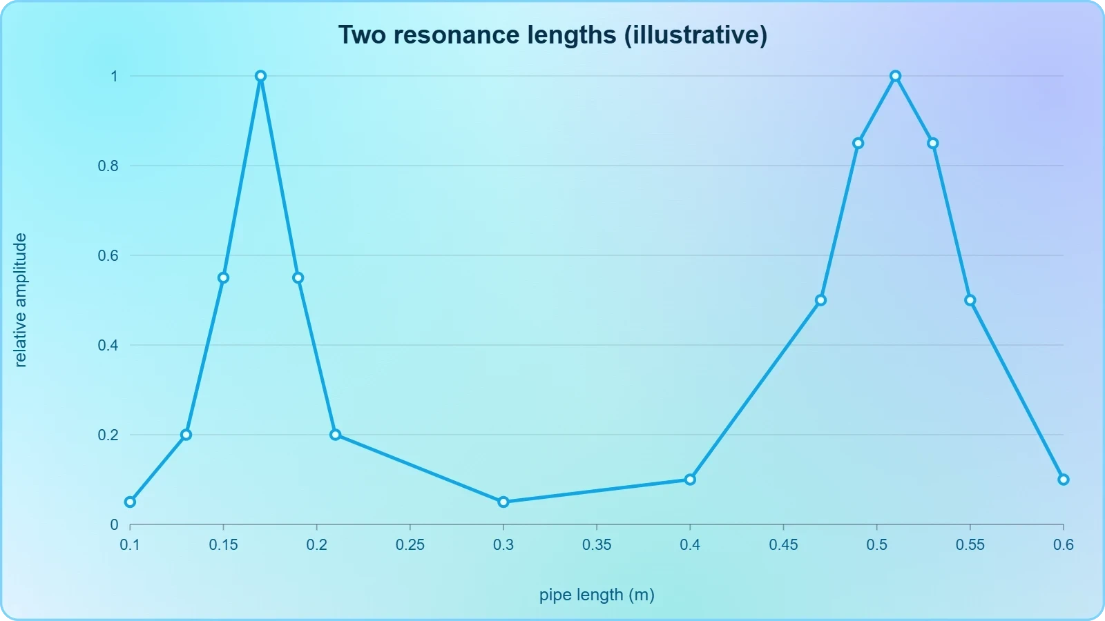
Had the measured lengths been ##0.16\ \text{m}## and ##0.50\ \text{m}##, the same difference would yield ##\lambda=0.68\ \text{m}## but an end correction of ##0.01\ \text{m}##. This illustrates the diagnostic power of the two-length method: the difference fixes the wavelength, while the absolute values reveal the correction. Examiners favour this structure because it tests both relations simultaneously.

Preparing for Resonance and Forced Vibrations

The standing waves derived here are natural modes, sustained without external driving once excited. The next lesson introduces an external periodic force and examines how the amplitude responds as the driving frequency approaches these natural frequencies. The sharpness of that response depends on damping, and the quality factor introduced earlier becomes the central parameter.

Recognising that resonance is simply forced excitation of a natural mode unifies the two lessons. Every result derived here, from ##f_n=nf_1## for strings to ##f=(2n-1)v/4L## for closed pipes, defines the frequencies at which a system will respond most strongly. The forthcoming treatment of forced oscillations will therefore build directly on this harmonic framework rather than introducing new physics.