Noise and Its Control

Noise is best defined not by its physical spectrum but by its reception: any sound that interferes with communication, rest, or concentration qualifies as unwanted, regardless of how orderly its waveform appears on an oscilloscope. This distinction matters for IIT JEE aspirants because the syllabus tests both the physics of sound intensity and the applied reasoning behind acoustic control, and examiners frequently blur the two. A pure 1000 Hz tone at 85 dB can be pleasant in one setting and intolerable in another, so the classification rests on context rather than frequency alone.

Lesson 16 builds directly on the harmonic analysis of musical instruments, where periodic overtones produce timbre, and extends that framework to aperiodic, irregular waveforms whose energy is spread across many frequencies without a stable pitch. That structural contrast—periodic versus random—is the physical foundation of everything that follows, from decibel arithmetic to the engineering of absorptive barriers. The lesson also prepares the ground for Lesson 17, which formalises sound intensity and pressure levels in greater mathematical depth.

Quantitative treatment is unavoidable here. The decibel scale compresses an enormous range of intensities into manageable numbers, and JEE problems routinely require logarithmic manipulation, superposition of multiple sources, and threshold comparisons. Health effects, meanwhile, introduce dose-response reasoning: exposure duration multiplies risk in ways that a single intensity reading cannot capture. The sections below move from measurement through physiological consequence to control engineering, closing with the problem patterns that recur in competitive examinations.

The Physics of Unwanted Sound: Measurement and Perception

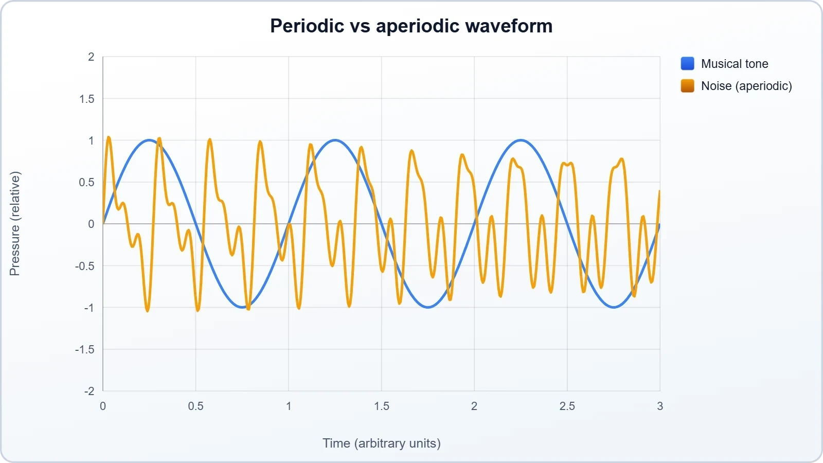
Sound becomes noise when its temporal structure loses periodicity, producing waveforms whose frequency content is continuous rather than discrete. Musical tones concentrate energy at a fundamental and its integer multiples; traffic, machinery, and crowd murmur distribute energy across a broad band with no stable harmonic series. This spectral distinction underpins every measurement technique discussed in this section and connects directly to the harmonic vocabulary established in the preceding lesson.

Intensity, the Decibel Scale, and Logarithmic Arithmetic

Sound intensity is power transmitted per unit area perpendicular to propagation, measured in watts per square metre. Because the audible range spans roughly fourteen orders of magnitude, engineers compress it logarithmically. The reference intensity corresponds to the threshold of hearing at 1000 Hz, and every tenfold increase in intensity adds a fixed number of decibels. This arithmetic is the single most examined quantitative idea in the lesson.

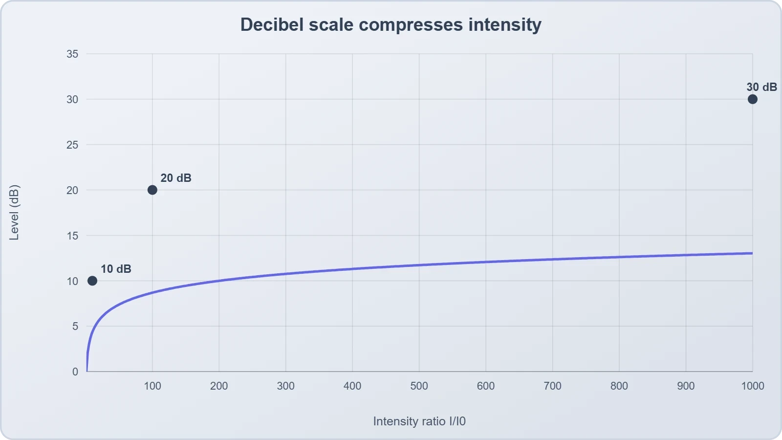
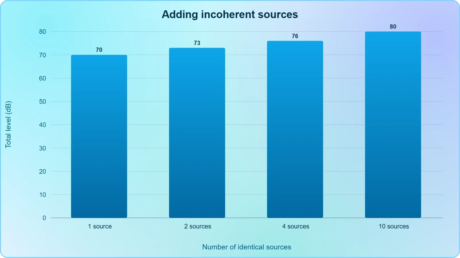
Two identical sources do not double the decibel value; they add three decibels, because intensity doubles while the logarithm converts the factor of two into ##10\log_{10}2 \approx 3.01##. Ten equal sources add ten decibels. JEE problems exploit this non-linearity constantly, asking students to combine sources, compare levels, or invert the relation to recover intensity ratios from stated decibel differences.

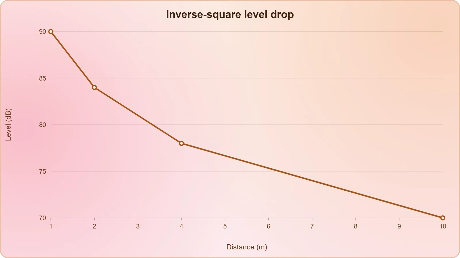
Distance introduces the inverse-square law for a point source radiating isotropically, so doubling the distance reduces intensity by a factor of four and the level by approximately six decibels. Real sources deviate from this ideal because of ground reflection, atmospheric absorption, and directivity, but the idealisation remains the examinable core. Students should practise chaining these relations: source power to intensity at a distance, then intensity to decibel level.

Frequency Weighting and the Loudness Curve

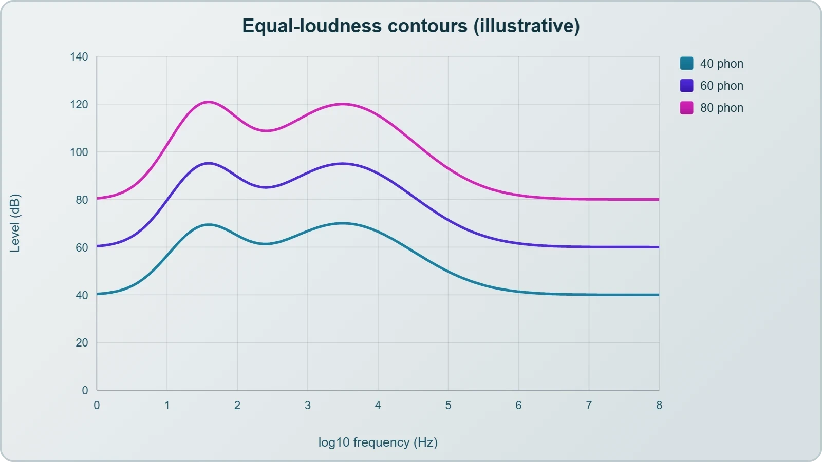
Human hearing is not equally sensitive across the spectrum; sensitivity peaks near three kilohertz and falls sharply at low frequencies. A-weighting filters measured spectra to approximate this response, producing the familiar dB(A) scale used in environmental regulation. Two sources with identical unweighted intensity can therefore differ substantially in perceived loudness, a point examiners test through qualitative comparison questions.

The equal-loudness contours, derived from systematic listening experiments, map combinations of frequency and intensity that sound equally loud. At low frequencies the curves steepen dramatically, meaning a fifty-hertz tone must carry far greater intensity than a three-kilohertz tone to be perceived at the same loudness. This explains why bass-heavy machinery feels physically intrusive despite modest measured levels.

For problem-solving, the practical consequence is that loudness comparisons require weighting assumptions to be stated explicitly. When a question supplies dB(A) values, the weighting is already embedded and no correction is needed. When it supplies raw intensities, students should note whether the comparison is physical or perceptual before selecting an approach.

Adding Sources and the Rules of Combination

Combining incoherent noise sources requires intensity addition, not amplitude addition, because random phases prevent systematic interference. Coherent tonal sources behave differently and can partially cancel, which is precisely why active noise cancellation works on periodic hum but struggles with broadband roar. Recognising whether sources are coherent or incoherent is the first decision in any combination problem.

A useful shortcut: when one source exceeds another by ten decibels or more, the quieter contributes negligibly to the total. This dominance rule saves time in multi-source questions and reflects the logarithmic compression directly. Students should verify it algebraically once, then apply it confidently under examination conditions.

Inverse-square spreading, absorption, and barrier attenuation each modify the level independently, and the standard examination approach multiplies the corresponding intensity factors before converting to decibels. Converting at the end rather than at each stage avoids compounding rounding errors. This discipline mirrors the intensity-and-pressure formalism developed in the following lesson.

Health Effects and the Physiology of Acoustic Exposure

Exposure consequences divide into auditory and non-auditory categories, and examination questions increasingly draw on both. Auditory damage arises from mechanical stress on the cochlea's hair cells, which do not regenerate in mammals; non-auditory effects include cardiovascular and cognitive responses mediated by stress pathways. The dose-response logic connecting them is the analytical thread of this section.

Temporary Threshold Shift and Permanent Hearing Loss

A brief exposure to loud sound elevates the threshold of audibility temporarily, a phenomenon called temporary threshold shift that resolves within hours or days. Repeated exposures without adequate recovery accumulate into permanent loss, particularly at the four-kilohertz notch where the cochlea is most vulnerable. The distinction between reversible and irreversible damage is a favourite conceptual question.

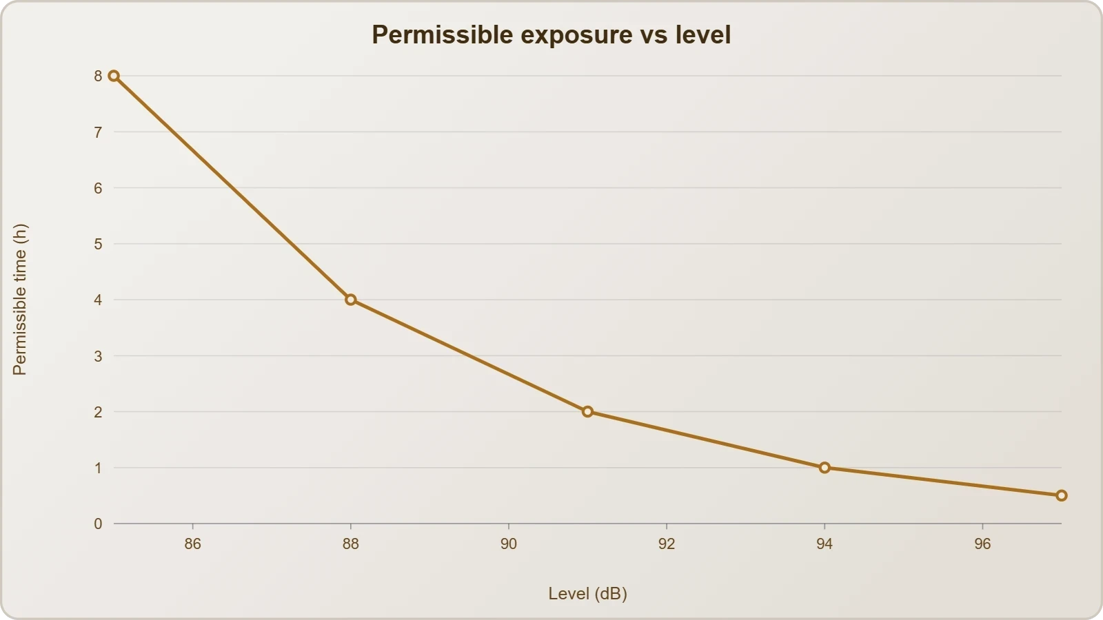
Risk scales with both intensity and duration, and occupational standards encode this through exchange rates: a three-decibel exchange rate halves permissible exposure time for every three-decibel increase. Under this rule, eighty-five decibels permits eight hours while eighty-eight decibels permits four. Students should be able to compute permissible durations across a range of levels using this halving logic.

Impulse noise from explosions or gunfire poses disproportionate risk because peak pressures can exceed one hundred forty decibels in milliseconds, overwhelming protective reflexes. The energy delivered in such transients can rival hours of continuous exposure. This asymmetry explains why impulse criteria in standards are stricter than continuous-noise criteria at comparable nominal levels.

Non-Auditory Consequences and Annoyance Metrics

Beyond the ear, chronic noise exposure correlates with elevated blood pressure, disturbed sleep architecture, and impaired concentration in learning environments. These effects appear at levels well below those causing hearing damage, which is why community noise limits are set near fifty-five decibels for residential areas. The evidence base is epidemiological rather than purely mechanistic, and questions may ask students to interpret such data critically.

Annoyance itself is quantified through survey-based metrics such as the percentage of a population highly annoyed, which rises steeply with night-time exposure. These social indicators drive policy more directly than laboratory physiology because they aggregate individual variability. Understanding the distinction between measured level and community response is essential for applied questions.

Cognitive performance studies in schools near airports show measurable deficits in reading comprehension attributable to aircraft noise, with effects persisting after controlling for socioeconomic factors. Such findings illustrate how dose-response reasoning extends beyond the laboratory into public health. Examiners occasionally frame questions around interpreting these observational studies.

Occupational Standards and Exposure Limits

Regulatory frameworks translate physiological evidence into enforceable limits, typically capping eight-hour average exposure at eighty-five decibels with a three-decibel exchange rate. Peak limits near one hundred forty decibels address impulse hazards separately. These figures recur in examination questions and should be memorised alongside their physiological justification.

Measurement practice matters as much as the limit itself: dosimeters worn on the body capture personal exposure, while fixed monitors characterise an area. The two can disagree substantially when workers move between zones. Questions sometimes probe this discrepancy, rewarding students who recognise that exposure is a property of the person, not the room.

Hearing protection attenuates incoming sound by a rated amount, but real-world protection is often less than the laboratory rating because of fit and wear time. The concept of effective protection, accounting for both attenuation and compliance, is a sophisticated point that distinguishes strong answers. It also links neatly to the engineering controls discussed next.

Control Strategies and Examination Problem Patterns

Noise control follows a hierarchy: reduce at source, interrupt the path, then protect the receiver. Engineering solutions at source are preferred because they eliminate exposure for everyone downstream, while personal protection is the last resort. This hierarchy structures both regulatory practice and the applied questions that appear in competitive papers, and it organises the final section of the lesson.

Source Reduction, Barriers, and Absorption

Source control includes improved machine design, vibration isolation mounts, and mufflers that dissipate acoustic energy before it radiates. Path control relies on barriers and enclosures whose effectiveness depends on mass per unit area and on sealing every gap, since a small opening can short-circuit an otherwise effective partition. These principles translate into quantitative questions about transmission loss.

Absorptive treatment inside a room reduces reverberant energy but does not block direct sound, a distinction students frequently confuse. Porous absorbers work best at mid and high frequencies, while low-frequency control demands greater thickness or resonant cavity designs. Matching absorber type to frequency band is a recurring applied question.

Barrier performance is limited by diffraction around edges, so a barrier must be large relative to the wavelength to be effective. This wavelength dependence explains why highway barriers work well against broadband traffic noise but poorly against low-frequency rumble. The diffraction reasoning connects back to the wave-optics material covered earlier in the course.

Active Cancellation and Receiver Protection

Active noise control generates an anti-phase signal that destructively interferes with the original, achieving substantial attenuation at low frequencies where passive absorbers are bulky. The technique works best for periodic, predictable noise such as engine hum and fails for broadband random sound because phase tracking becomes impossible. This coherence requirement links directly to the source-combination rules established earlier.

Receiver protection includes earplugs, earmuffs, and administrative controls such as rotation that limit individual exposure duration. Combining protection with rotation is common in industry, and questions may ask students to compute effective exposure under a mixed schedule. The arithmetic mirrors the dose calculations already practised.

Hearing conservation programmes combine monitoring, protection, and audiometric testing, reflecting the recognition that no single measure suffices. This systems view is worth stating explicitly in descriptive answers, where examiners reward integrated reasoning over isolated facts. It also anticipates the intensity formalism of the next lesson.

Worked Problem Patterns for JEE

Typical problems ask for the level at a distance given source power, the combined level of several sources, or the intensity ratio implied by a stated decibel difference. Each reduces to careful logarithmic manipulation with the reference intensity fixed. Practising the inversion from level to intensity builds the fluency these questions demand.

import math

def level_from_intensity(intensity):
    # Reference intensity for air at 1000 Hz
    i0 = 1e-12
    return 10 * math.log10(intensity / i0)

def combine_incoherent(levels):
    # Convert each level to intensity, sum, then convert back
    i0 = 1e-12
    total = sum(i0 * 10 ** (L / 10) for L in levels)
    return 10 * math.log10(total / i0)

print(round(level_from_intensity(1e-5), 2))        # 70.0 dB
print(round(combine_incoherent([70, 70]), 2))      # 73.01 dB
print(round(combine_incoherent([90, 70]), 2))      # 90.04 dB

The final example illustrates the dominance rule numerically: a seventy-decibel source adds only four hundredths of a decibel to a ninety-decibel source. Students who internalise this pattern avoid unnecessary computation under time pressure. The same logic extends to any number of sources once intensities are summed correctly.

A second pattern involves distance: given a level at one metre, find the level at ten metres under inverse-square spreading. The intensity falls by a factor of one hundred, so the level drops by twenty decibels. Chaining this with barrier attenuation and absorption produces the multi-step questions that separate strong candidates.