Advanced Problem Solving in Sound

Lesson 29 of this thirty-part IIT JEE series arrives at the point where isolated formulas stop being sufficient. Advanced sound problems rarely test a single principle; they fuse standing-wave boundary conditions, Doppler shifts, resonance geometry, and intensity bookkeeping into a single stem that must be decomposed before any algebra begins. The preceding lesson on psychoacoustics established how the ear interprets frequency and loudness, and that perceptual framing now becomes a diagnostic tool rather than a curiosity.

JEE Advanced papers consistently reward candidates who recognise structural patterns before computing. A pipe problem that mentions a moving source, a temperature change, and a beat frequency is not three separate questions; it is one wave equation constrained by three boundary conditions applied in sequence. This lesson therefore treats problem-solving as a discipline of classification, variable isolation, and dimensional verification, with worked derivations that mirror the examination's actual difficulty gradient.

Because the next lesson consolidates the entire course into revision, the material here deliberately avoids repetition of earlier derivations. Instead, it assembles them under pressure: multi-concept stems, superposition of travelling and standing waves, end-correction subtleties in organ pipes, and Doppler configurations involving reflection and moving media. Each section supplies the reasoning scaffold, the governing equations in MathJax form, and the numerical discipline that converts a plausible answer into a defensible one.

Deconstructing Multi-Concept Stems in Advanced Sound Problems

Advanced stems are engineered so that no single equation yields the answer. The examiner embeds a constraint that silently fixes one variable, then asks for a quantity that depends on it through two intermediate relations. Recognising which constraint is binding, and in what order the relations must be applied, separates a four-minute solution from a fifteen-minute dead end.

Classifying the Problem Before Computing

Every advanced sound question belongs to a small family: resonance in bounded media, interference and beats, Doppler kinematics, or intensity and energy transport. Classification should occur within the first thirty seconds of reading. Once the family is identified, the relevant boundary conditions and sign conventions follow automatically, and the candidate avoids the common error of importing a formula from the wrong family.

A useful discipline is to annotate the stem physically before writing symbols. Mark which medium is moving, which observer is stationary, whether the pipe is open or closed, and whether the source approaches or recedes. These annotations determine the sign structure of the Doppler relation and the harmonic index of the standing wave, both of which are frequent sources of silent arithmetic error under examination pressure.

Classification also exposes redundant information. Advanced stems often include a datum that is never needed, inserted to test whether the candidate understands which variables are independent. A candidate who computes every quantity mentioned wastes time; one who identifies the minimal variable set reaches the answer faster and with fewer opportunities for arithmetic slip.

Finally, classification determines the expected order of magnitude. A fundamental frequency for a metre-long air column near room temperature sits in the low hundreds of hertz, so an answer of 40 Hz or 4,000 Hz signals a unit or harmonic-index error. This sanity check costs seconds and catches mistakes that algebra alone will not reveal.

Variable Isolation and Dimensional Verification

Once classified, the problem reduces to isolating the target variable through a chain of substitutions. The governing relations for sound are few: wave speed ##v = f\lambda##, standing-wave conditions for pipes, beat frequency ##f_{beat} = |f_1 - f_2|##, and the Doppler relation for a moving source or observer. Chaining them requires care with units at every step.

Dimensional verification should be applied to every intermediate expression, not only the final answer. If an intermediate quantity is claimed to be a frequency but carries dimensions of length, the substitution order is wrong. This check is especially valuable when temperature corrections enter, because the speed of sound depends on absolute temperature as ##v \propto \sqrt{T}##, and mixing Celsius with Kelvin silently corrupts the result.

Symbolic isolation before numerical substitution is the safer strategy. Solving for the target in symbols exposes cancellations, reduces rounding accumulation, and makes the dimensional structure transparent. Only after the symbolic form is verified should numerical values be inserted, ideally with a single final calculation rather than a chain of rounded intermediates.

Where a problem admits two algebraic roots, physical reasoning must select between them. A beat frequency, for instance, gives an absolute difference and therefore two candidate source frequencies; the direction of the beat change when loading is altered resolves the ambiguity. Advanced problems frequently hinge on exactly this kind of disambiguation.

Worked Example: Pipe, Temperature, and Beats Combined

Consider a closed organ pipe whose fundamental at 27 °C matches a tuning fork, and which produces three beats per second when the air is heated. The speed of sound scales as the square root of absolute temperature, so the pipe frequency rises with heating. Since the beat count increases, the pipe frequency must move away from the fork, fixing the fork below the original pipe frequency.

The arithmetic follows directly. At 300 K the pipe fundamental is ##f_0##; at the elevated temperature ##T##, the fundamental becomes ##f_0\sqrt{T/300}##. The beat condition gives ##f_0\sqrt{T/300} - f_{fork} = 3## with ##f_{fork} = f_0 - 3##, which yields a single equation in ##T## once ##f_0## is supplied by the pipe geometry.

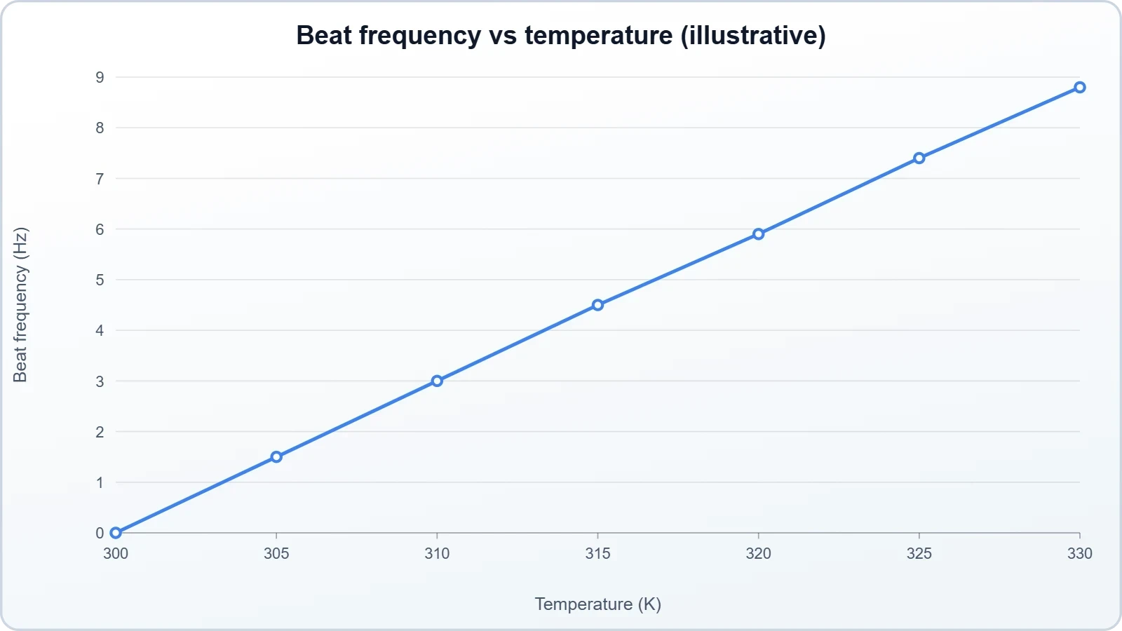
The lesson generalises: whenever a stem couples geometry, thermodynamics, and interference, the correct strategy is to express each physical effect as a multiplicative or additive modification of a base frequency, then impose the interference condition last. This ordering keeps the algebra linear and the physical interpretation intact throughout.

Superposition, Standing Waves, and Resonance Under Examination Conditions

Superposition is the conceptual hinge of the entire course, and advanced problems exploit it in compound form. Two travelling waves of slightly different frequency produce beats; identical counter-propagating waves produce standing patterns; partial reflection inside a pipe produces both simultaneously. The candidate must track which superposition is active at each boundary and which quantity the question actually requests.

End Corrections and Real Pipe Behaviour

Ideal pipe formulas assume pressure nodes exactly at the open end, but real air columns extend slightly beyond the rim. The end correction ##e \approx 0.6r## for a single open end shifts every harmonic upward and becomes measurable when pipes of different radii are compared. Advanced problems exploit this by asking which of two pipes resonates first.

The corrected condition for a closed pipe becomes ##f_n = (2n-1)v/[4(L + e)]##, and for an open pipe ##f_n = nv/[2(L + 2e)]##. The asymmetry between one and two corrections is a favourite trap: candidates who apply the same correction to both configurations obtain a systematically wrong ratio and lose the comparison question entirely.

End correction also explains why a tuning fork held over a resonance tube yields successive resonances whose spacing is ##\lambda/2## while the first occurs near ##\lambda/4##. The difference between the first and second resonance positions, doubled, gives the wavelength directly, and the residual offset yields the end correction without any separate measurement.

In examination settings, end corrections are usually small enough to be neglected unless explicitly mentioned. The disciplined approach is to check whether the stem supplies a radius or a measured first-resonance position; if it does, the correction is intended to be used, and ignoring it forfeits the marks allocated to that subtlety.

Resonance Chains and Coupled Conditions

Resonance problems become genuinely advanced when two conditions must hold simultaneously. A string vibrating in sympathy with an air column, or a pipe whose length is adjusted until beats vanish against a fork, imposes two equations on the same frequency. Solving requires expressing both systems in terms of a common variable, usually the shared frequency or the wave speed.

The general method is to write each subsystem's resonance condition independently, then equate the frequencies. For a string of tension ##T_s## and linear density ##\mu##, ##f = \dfrac{n}{2L_s}\sqrt{T_s/\mu}##; for the pipe, the harmonic condition supplies the second expression. Equating them and isolating the unknown tension or length completes the solution.

Advanced variants add a constraint that the resonance must be the lowest possible, or that a specified number of beats must be heard. These constraints select the harmonic indices ##n## and ##m##, which are otherwise free. The candidate must therefore test small integer pairs systematically rather than assuming fundamentals throughout.

A final subtlety concerns energy transfer. At resonance the coupled system absorbs energy efficiently, and the amplitude grows until damping balances the input. Questions occasionally ask about the amplitude ratio or the quality factor, which requires recognising that resonance is a steady-state energy balance, not merely a frequency coincidence.

Interference Geometry and Path Differences

Two-source interference in air follows the same path-difference logic as light, but the longer wavelength makes the geometry experimentally accessible. Constructive interference requires ##\Delta r = m\lambda## and destructive interference ##\Delta r = (m + \tfrac{1}{2})\lambda##, with the phase of each source included when the sources are not in phase.

Advanced problems often place the observer off the axis, converting a one-dimensional beat question into a two-dimensional path-difference calculation. The distance from each source to the observation point must be computed geometrically, and the difference compared with the wavelength. Small-angle approximations are valid only when the observer is far compared with the source separation.

When the sources differ in phase by ##\phi##, the conditions shift: constructive interference occurs at ##\Delta r = (m - \phi/2\pi)\lambda##. This phase offset is frequently hidden in the stem as a description of how the sources are driven, and candidates who ignore it obtain a pattern displaced by half a fringe.

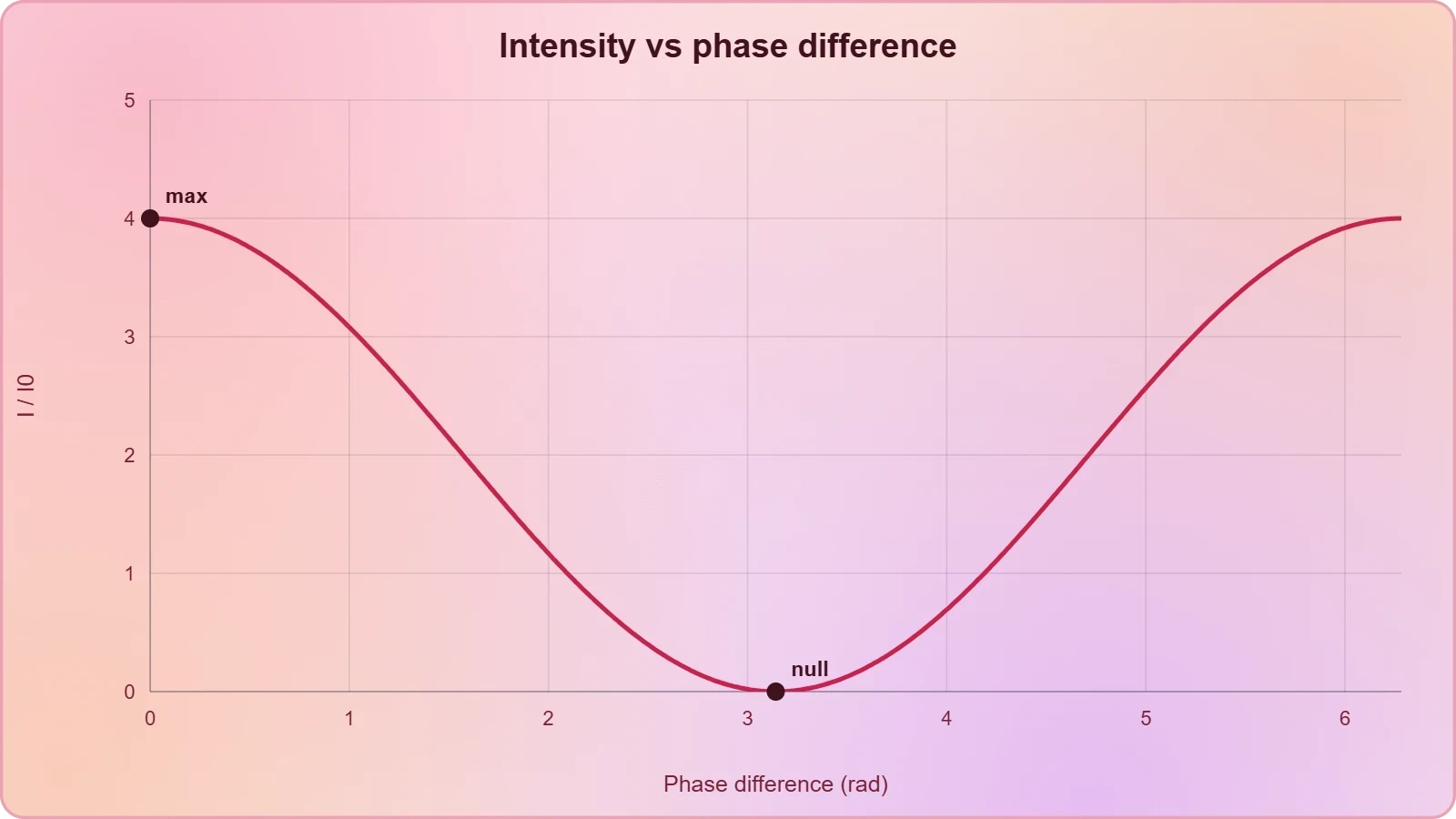
Intensity at the observation point follows from coherent superposition: ##I = I_1 + I_2 + 2\sqrt{I_1 I_2}\cos\delta##, where ##\delta## is the total phase difference. This relation explains why equal sources produce a contrast ratio of four to zero and why unequal sources never fully cancel, a point advanced questions test directly.

Doppler Kinematics and Intensity Calculations in Compound Scenarios

The Doppler effect is the most heavily examined topic in advanced sound papers because it combines kinematics with wave propagation and admits many sign configurations. The general relation for a source and observer moving along the line joining them is straightforward, but reflection, moving media, and perpendicular motion generate variants that punish memorisation and reward derivation from first principles.

Sign Conventions and the General Doppler Relation

The standard relation for a stationary medium is ##f' = f\dfrac{v \pm v_o}{v \mp v_s}##, where the upper signs correspond to approach. The convention is easiest to remember physically: approach raises the observed frequency, recession lowers it. Every sign choice should be checked against this physical expectation before the arithmetic proceeds.

Advanced problems frequently involve motion at an angle to the line of sight. Only the component of velocity along the source-observer line contributes to the first-order shift, so the effective velocities are ##v_s\cos\theta_s## and ##v_o\cos\theta_o##. Perpendicular motion produces no first-order shift, a result that surprises candidates who expect any motion to alter pitch.

When the medium itself moves, as with wind, the wave speed relative to the ground changes while the frequency in the medium is set by the source. The correct approach is to transform into the medium's frame, apply the standard relation, and transform back. Wind blowing from source to observer raises the observed frequency; wind in the opposite direction lowers it.

Reflection problems add a second Doppler step. A wave emitted by a moving source, reflected by a moving wall, and received by a moving observer undergoes two successive shifts, each governed by the relation with the appropriate velocities. The composite shift is the product of the two factors, not their sum, and this multiplicative structure is a recurring examination point.

Reflection, Moving Walls, and Echo Problems

Echo problems are Doppler problems in disguise. A stationary source emits toward a moving wall; the wall receives a shifted frequency and re-emits it as a moving source. The observer then receives a second shift. The beat frequency between the emitted and received signals encodes the wall's velocity and is the quantity usually requested.

For a wall approaching with speed ##u##, the received frequency at the wall is ##f_1 = f\dfrac{v+u}{v}##, and the frequency returning to the stationary source is ##f_2 = f_1\dfrac{v}{v-u}##. The beat frequency is ##f_2 - f_1##, which for small ##u## reduces to approximately ##2fu/v##, a result worth memorising as a check.

When both source and wall move, the two shifts must be applied in the correct order and with the correct signs. The disciplined method is to label each propagation leg, assign velocities relative to the medium, and apply the relation leg by leg. Skipping a leg or reversing a sign produces an answer that is dimensionally correct but physically wrong.

Sonar and radar variants replace the acoustic wave with an electromagnetic one, but the same two-leg structure applies with the appropriate wave speed. The acoustic case is examined more often in JEE because the medium matters, and the medium's motion relative to the ground introduces an additional degree of freedom that the electromagnetic case lacks.

Intensity, Decibels, and Energy Transport

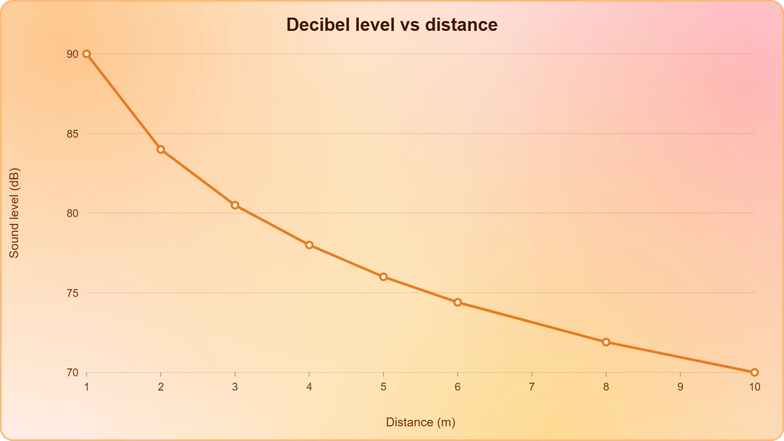
Intensity problems test whether the candidate understands that sound energy spreads geometrically. For a point source in free space, ##I = P/(4\pi r^2)##, so intensity falls as the inverse square of distance. Two sources of equal power produce double the intensity but only a modest increase in loudness, because the ear responds logarithmically.

The decibel scale is defined as ##L = 10\log_{10}(I/I_0)## with ##I_0 = 10^{-12}\ \text{W/m}^2##. Advanced questions combine this with the inverse-square law: moving from one metre to ten metres reduces intensity by a factor of one hundred, which corresponds to a twenty-decibel drop. Such combinations are common and reward fluency with logarithms.

When multiple incoherent sources overlap, intensities add directly; when coherent, amplitudes add and interference terms appear. The distinction is physical, not mathematical, and the stem usually signals it by describing the sources as independent or as driven from a common oscillator. Misclassifying the coherence changes the answer by a factor of two or more.

Energy transport questions occasionally ask for the total power crossing a surface or the energy density in a standing wave. The intensity of a plane wave is ##I = \tfrac{1}{2}\rho v \omega^2 A^2##, where ##A## is the displacement amplitude. This relation links the mechanical description of the wave to the energetic one and is the natural bridge to the revision lesson that follows.

Numerical Discipline and Common Traps

Advanced sound problems are lost more often to arithmetic and unit errors than to conceptual gaps. The speed of sound at room temperature is approximately 340 m/s, and using 330 or 350 without justification can shift an answer beyond the tolerance of the options. Stating the assumed value explicitly protects the solution.

Temperature, as noted, must be in kelvin. A stem quoting 27 °C requires 300 K, and the square-root dependence means a ten-kelvin error produces roughly a 1.7 percent frequency error, which is often enough to change the selected option. This is the single most common silent error in thermal-acoustic problems.

Harmonic indices are the second trap. Closed pipes support only odd harmonics, so the third resonance corresponds to ##n = 3## in the odd series, not the third harmonic of an open pipe. Candidates who carry open-pipe intuition into closed-pipe problems systematically misidentify the harmonic and lose the question.

Finally, answers should be checked against limiting cases. If a moving source's speed tends to zero, the Doppler shift must vanish; if the observer recedes at the wave speed, the observed frequency must tend to zero. These limits are quick to evaluate and catch sign errors that survive dimensional analysis.

Structuring a Full-Marks Solution

JEE Advanced awards partial credit for method, so the written solution should expose the reasoning chain. Begin with a labelled diagram, state the governing relations symbolically, substitute only at the end, and box the final answer with units. This structure also makes self-checking faster during the examination.

Time allocation matters as much as correctness. A multi-concept sound problem should consume roughly six to eight minutes; beyond that, the marginal return falls below the cost of abandoning it. Practising under timed conditions builds the judgement needed to decide when to persist and when to move on.

Reviewing past papers reveals that the same structural patterns recur with different numbers. The pipe-temperature-beat combination, the moving-wall echo, and the two-source interference geometry account for a large fraction of advanced sound questions. Recognising these patterns is the practical payoff of the classification discipline introduced earlier.

This lesson closes the technical content of the course. The final lesson consolidates the full syllabus into revision notes, formula sheets, and a timed mock, drawing on every principle developed here. Candidates who have internalised the classification and verification habits are well positioned for that consolidation.

import math

def closed_pipe_frequency(L, T_celsius, harmonic=1, end_correction=0.0):
    v0, T0 = 343.0, 293.15
    v = v0 * math.sqrt((T_celsius + 273.15) / T0)
    return (2 * harmonic - 1) * v / (4 * (L + end_correction))

def beat_frequency(f1, f2):
    return abs(f1 - f2)

def doppler(f, v, v_obs, v_src):
    # positive velocities mean approach
    return f * (v + v_obs) / (v - v_src)

f_pipe = closed_pipe_frequency(0.5, 27.0)
f_shifted = doppler(f_pipe, 343.0, 0.0, 10.0)
print(round(f_pipe, 2), round(f_shifted, 2), round(beat_frequency(f_pipe, f_shifted), 2))

The script above encodes the three relations most often chained in advanced problems, and running it against a sample configuration confirms the expected order of magnitude. Candidates who can reproduce such a script mentally, without the interpreter, have internalised the structure that the examination rewards.