Doppler Effect for Sound

The Doppler effect describes the systematic shift in observed frequency when a wave source and an observer move relative to the medium carrying the wave. For sound, the medium is air, and this detail matters enormously: unlike light, sound requires a material medium, so velocities must be measured against the air frame rather than simply against each other. This lesson isolates that principle and applies it to the three canonical configurations examined in IIT JEE papers.

Building directly on the beats lesson, where two slightly detuned sources produced an amplitude envelope at the difference frequency, we now allow relative motion to generate the frequency difference itself. A single moving source can produce the same audible beating against a stationary reference tone that two static sources produced previously. This continuity is deliberate: the physics of superposition remains intact, but the frequency entering the superposition now depends on kinematics.

The treatment proceeds from the general Doppler formula through moving-source, moving-observer, and combined cases, closing with medium-wind corrections and JEE-style problem strategy. Each configuration is derived from wavefront geometry rather than memorised, because examination questions routinely invert the standard setup. By the end, you should be able to assign signs correctly under time pressure and connect this material to the intensity and loudness discussion that follows.

The Doppler Effect for Sound: Core Principles and the General Frequency Formula

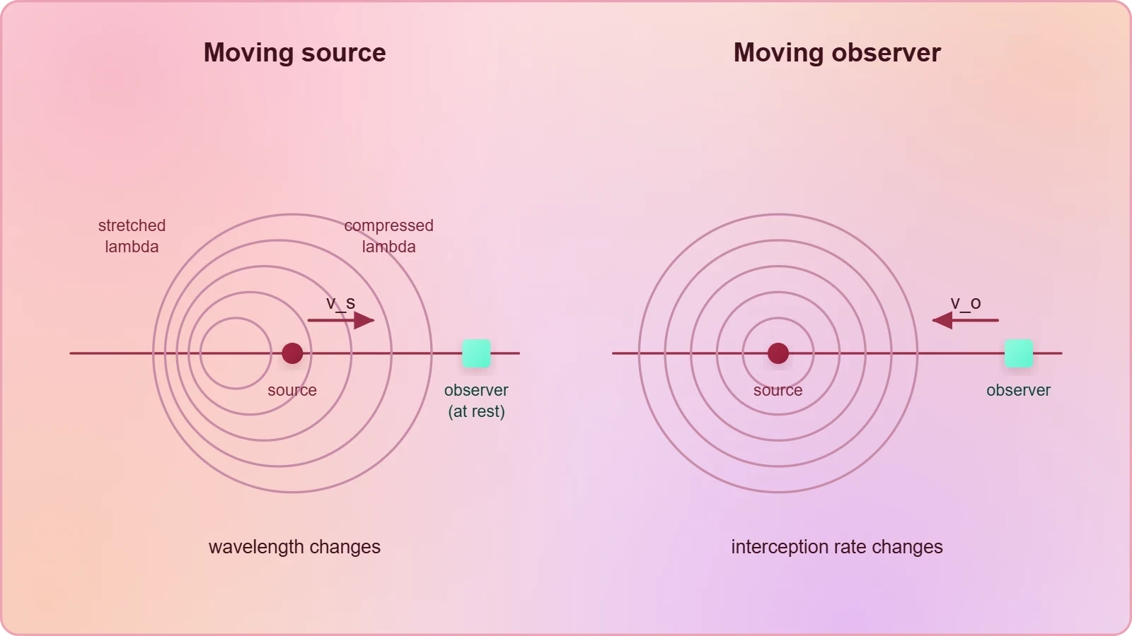
The Doppler shift for sound arises because relative motion changes either the wavelength in the medium, the rate at which wavefronts are intercepted, or both simultaneously. A source advancing through air compresses successive wavefronts ahead of it and stretches them behind, altering the spatial periodicity that a stationary observer samples. An observer moving through the wave field instead changes the temporal rate of interception without altering the wavelength at all.

This separation of mechanisms is the conceptual anchor for the entire lesson. Wavelength is a property of the medium and the source motion; interception rate is a property of the observer motion. Confusing the two is the single most common error in examination attempts, and it produces sign errors that propagate through every subsequent calculation.

Deriving the General Doppler Expression

Consider a source emitting at frequency ##f_0## and wavelength ##\lambda = v/f_0## in still air, where ##v## is the sound speed, approximately 343 m/s at 20 °C. If the source moves toward a stationary observer at speed ##v_s##, each successive wavefront is emitted from a position closer to the observer, compressing the wavelength to ##\lambda' = (v - v_s)/f_0##.

The observer, stationary in the medium, intercepts these compressed wavefronts at the unchanged speed ##v##, so the observed frequency becomes ##f' = v/\lambda' = f_0 \, v/(v - v_s)##. This is the moving-source result: approach raises the observed pitch, and recession lowers it, with the shift growing nonlinearly as ##v_s## approaches ##v##.

Now let the observer move toward a stationary source at speed ##v_o##. The wavelength in air remains ##v/f_0##, but the observer closes on wavefronts at relative speed ##v + v_o##, giving ##f' = f_0 (v + v_o)/v##. Combining both motions yields the general formula that governs every configuration in this lesson.

The sign convention is mechanical rather than mysterious: choose the upper signs in the numerator and denominator to represent approach, and the lower signs to represent recession. Equivalently, assign positive velocity to motion that reduces the source–observer separation. Consistency in applying this rule eliminates most errors, provided the velocities are measured relative to the air.

Why the Medium Frame Matters

Because sound propagates through air, the air frame is the privileged reference frame for the Doppler formula. A source and observer approaching each other at identical speeds do not produce symmetric shifts: the moving-source term appears in the denominator and amplifies nonlinearly, while the moving-observer term appears in the numerator and acts linearly. This asymmetry has no counterpart in relativistic light Doppler shifts.

Wind complicates the picture by shifting the effective medium frame. If wind blows at speed ##w## toward the observer, the sound speed relative to the ground becomes ##v + w##, and all velocities in the formula must be re-expressed relative to the moving air. Examination questions occasionally test this, and the correct procedure is always to transform into the air frame first.

Limiting Cases and the Sonic Boundary

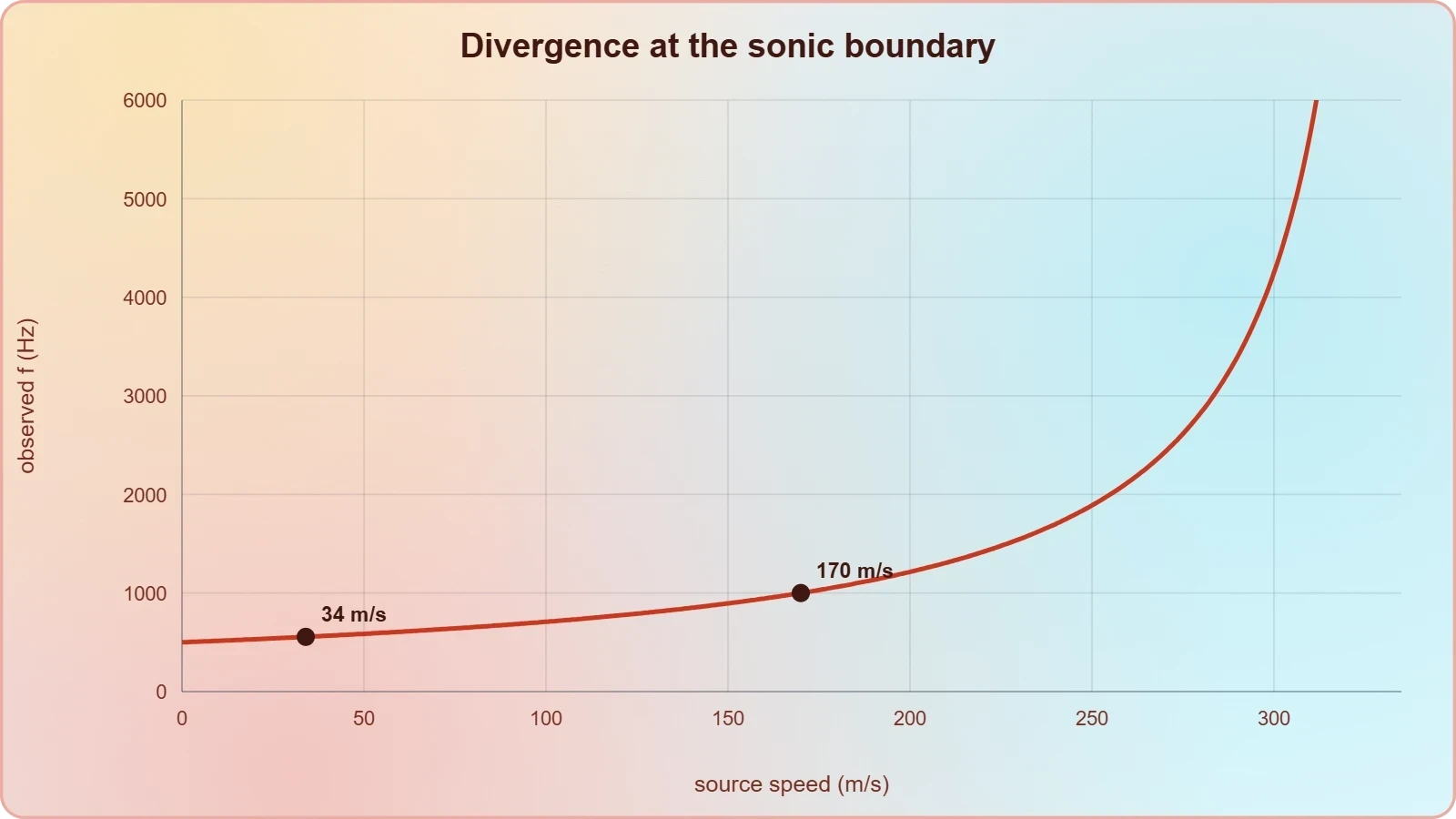
As ##v_s \to v##, the denominator approaches zero and the observed frequency diverges, signalling the formation of a shock front rather than an infinite pitch. Beyond this speed the source outruns its own wavefronts, producing a Mach cone with half-angle given by ##\sin\theta = v/v_s##. This regime lies outside standard JEE scope but clarifies why the formula fails.

Conversely, when ##v_s = 0## and ##v_o = 0##, the formula collapses to ##f' = f_0##, as required. Testing these limits is a rapid sanity check during examinations, and it catches sign errors before they consume valuable solving time on multi-part questions.

Worked Configurations: Moving Source, Moving Observer, and Combined Motion

Applying the general formula to concrete configurations develops the fluency that timed examinations demand. The three canonical cases below are presented with numerical values chosen to reflect realistic JEE parameters, and each is solved by explicit substitution rather than pattern matching. Pay attention to how the sign assignment follows directly from the geometry of approach or recession.

Case One: The Moving Source

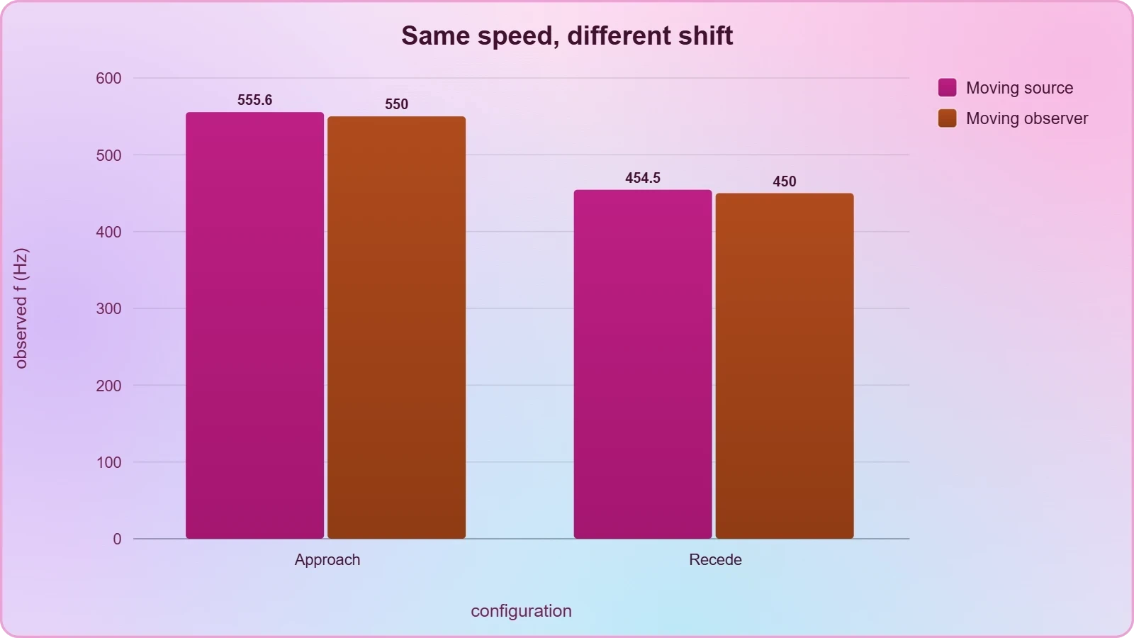
A train sounding a 500 Hz horn approaches a stationary platform observer at 34 m/s, with sound speed 340 m/s. Substituting into the moving-source form gives ##f' = 500 \times 340/(340 - 34) = 500 \times 340/306 \approx 555.6## Hz. The pitch rises by roughly 11 percent, a shift clearly audible to the human ear.

After passing, the same train recedes at 34 m/s, and the formula yields ##f' = 500 \times 340/374 \approx 454.5## Hz. The total swing across the pass is approximately 101 Hz, and the drop occurs abruptly at the moment of closest approach. This discontinuity in observed frequency is the signature of a moving source.

Note the asymmetry: the upward shift of 55.6 Hz exceeds the downward shift of 45.5 Hz. This follows from the nonlinearity of the denominator, and it explains why the classic passing-train pitch drop sounds steeper than a naive linear estimate would predict. Examiners exploit this asymmetry in conceptual multiple-choice items.

A useful approximation for small source speeds, ##v_s \ll v##, is ##\Delta f/f_0 \approx v_s/v##, giving about 10 percent here against the exact 11.1 percent. The approximation is worth memorising for rapid estimation, but exact substitution should be used whenever the answer options are closely spaced.

Case Two: The Moving Observer

An observer in a car moving at 34 m/s toward a stationary 500 Hz siren hears ##f' = 500 \times (340 + 34)/340 = 500 \times 374/340 = 550## Hz. Compare this with the 555.6 Hz obtained for an identical source speed: the moving observer experiences a smaller shift than the moving source, despite identical relative speed.

Receding at the same speed, the observer hears ##f' = 500 \times 306/340 = 450## Hz. The upward and downward shifts are now symmetric at 50 Hz each, in contrast to the moving-source case. This symmetry is a direct consequence of the linear numerator and provides a clean diagnostic for identifying which object is moving.

This distinction is frequently tested through questions that specify only the relative velocity and ask which configuration produces the larger shift. The answer is always the moving source, because the denominator amplifies the effect. Recognising this saves substantial time when the question is qualitative rather than numerical.

Physically, the moving observer intercepts more wavefronts per second without altering the wave field, whereas the moving source actually compresses the wave field itself. The medium records the difference, and any detector placed in the air will confirm that the wavelength genuinely differs between the two cases.

Case Three: Combined Motion

When both move, substitute both velocities with independently assigned signs. A source approaching at 20 m/s while the observer approaches at 30 m/s, with ##f_0 = 600## Hz and ##v = 340## m/s, gives ##f' = 600 \times (340 + 30)/(340 - 20) = 600 \times 370/320 \approx 693.8## Hz.

If instead the observer recedes at 30 m/s while the source still approaches, the numerator becomes ##340 - 30 = 310##, yielding ##f' = 600 \times 310/320 \approx 581.3## Hz. The observed frequency can therefore rise or fall even while the source approaches, depending on the observer's motion.

Care is needed when the two move in the same direction at different speeds. Transform each velocity into the air frame, then apply the formula; do not subtract the speeds and treat the result as a single relative velocity. This shortcut works only in the special case where one body is stationary in the medium.

A common examination trap involves a source chasing an observer who is moving away faster than the source. Here the separation increases, so the observed frequency falls below ##f_0## despite both moving in the same direction. Assigning signs from the separation rate, rather than from direction labels, resolves the ambiguity reliably.

Problem-Solving Strategy, Medium Corrections, and Examination Applications

Examination performance on Doppler questions depends less on algebra than on disciplined setup. The recommended sequence is to identify the medium frame, assign signs from the rate of change of separation, substitute into the general formula, and verify the limiting behaviour. Each step is quick, and together they eliminate the sign errors that account for most lost marks in this topic.

Beyond mechanics, the Doppler effect connects to a wide range of physical applications, from radar speed measurement to medical ultrasound flow imaging and astronomical redshift. While the light-Doppler formula differs because no medium exists, the sound case remains the conceptual foundation, and JEE questions occasionally ask students to contrast the two regimes qualitatively.

A Systematic Solution Protocol

Begin by writing the general formula explicitly before substituting any numbers. This forces conscious sign selection and prevents the common habit of plugging values into a half-remembered variant. Mark the direction of each velocity on a simple diagram, then translate the diagram into signs using the separation-rate rule.

Next, check that all velocities are expressed in the air frame. If wind is present, add or subtract the wind velocity from both source and observer speeds before substitution. Finally, verify that the answer lies on the correct side of ##f_0##: approach must yield ##f' > f_0##, and recession must yield ##f' < f_0##.

For multi-part questions, compute the frequency at closest approach and at the specified positions separately rather than attempting a single combined expression. This modular approach reduces algebraic clutter and makes partial credit more likely when one segment contains an arithmetic slip. It also mirrors the structure of the physical situation.

Where the question supplies a beat frequency between the Doppler-shifted sound and a reference tone, recall from the previous lesson that ##f_{beat} = |f' - f_{ref}|##. The Doppler shift supplies ##f'##, and the beat relation then determines the unknown velocity. This linkage between consecutive lessons is a favourite of paper setters.

Wind, Medium Motion, and the Air Frame

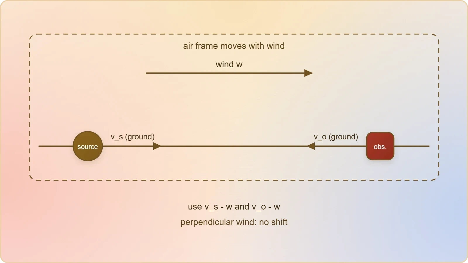
When wind blows at velocity ##w## along the source–observer line, the sound speed relative to the ground is ##v + w## for propagation downwind. The general formula remains valid provided every velocity is measured in the air frame, which requires subtracting ##w## from each ground-frame velocity before substitution.

A subtle consequence is that wind alone, with both source and observer stationary on the ground, produces no frequency shift. The wavelength and the interception rate change together in a way that cancels exactly. This null result is a useful conceptual checkpoint and occasionally appears as a true-or-false item.

If the wind blows perpendicular to the line of sight, the component along the propagation direction is zero to first order, and the shift is negligible. Only the longitudinal component of medium motion enters the formula, which simplifies most practical problems to a one-dimensional correction.

Students should also recognise that the medium frame is not always the ground frame in laboratory problems. In a wind tunnel or a moving vehicle carrying both source and detector, the air may be stationary relative to the apparatus, and the formula applies without correction. Reading the problem statement carefully determines which frame is appropriate.

Applications and the Bridge to Intensity

Radar and sonar speed guns exploit the Doppler shift to measure approaching vehicles and submarines, while medical ultrasound uses the same principle to map blood flow velocity through vessels. In each case, the measured frequency shift converts directly into a velocity through the general formula, inverted algebraically.

Astronomical redshift applies the light-Doppler relation rather than the sound formula, but the conceptual parallel is instructive. Because light requires no medium, only the relative velocity matters, and the relativistic factor appears. JEE questions sometimes ask students to identify this distinction explicitly.

The next lesson turns to intensity and loudness, where the amplitude and energy transport of sound waves take centre stage. The Doppler effect changes frequency, not intensity, so the two topics are complementary rather than overlapping. Together they complete the treatment of what a listener actually perceives.

Before proceeding, consolidate the sign convention through repeated practice on mixed configurations. Fluency here pays dividends across the remaining lessons, particularly in questions that combine Doppler shifts with beat frequencies or resonance conditions in pipes and strings.

def doppler_frequency(f0, v, v_source, v_observer, approach=True):
    """Compute observed frequency for sound Doppler effect.
    Velocities are magnitudes in the air frame (m/s)."""
    if approach:
        return f0 * (v + v_observer) / (v - v_source)
    return f0 * (v - v_observer) / (v + v_source)

v = 340.0
print(round(doppler_frequency(500, v, 34, 0, True), 1))   # 555.6 Hz
print(round(doppler_frequency(500, v, 0, 34, True), 1))   # 550.0 Hz
print(round(doppler_frequency(500, v, 34, 0, False), 1))  # 454.5 Hz