The Human Genome Project did not merely deliver a string of letters three billion characters long; it delivered a new way of seeing human biology. When the first drafts were announced in 2001 and the finished sequence followed in 2003, researchers confronted a landscape that overturned several comfortable assumptions. The genome turned out to be smaller in gene count, richer in repetitive sequence, and far more uniform between individuals than anyone had predicted. Those three surprises, taken together, reframed genetics from a discipline of counting genes to a discipline of understanding regulation, variation, and evolutionary history.
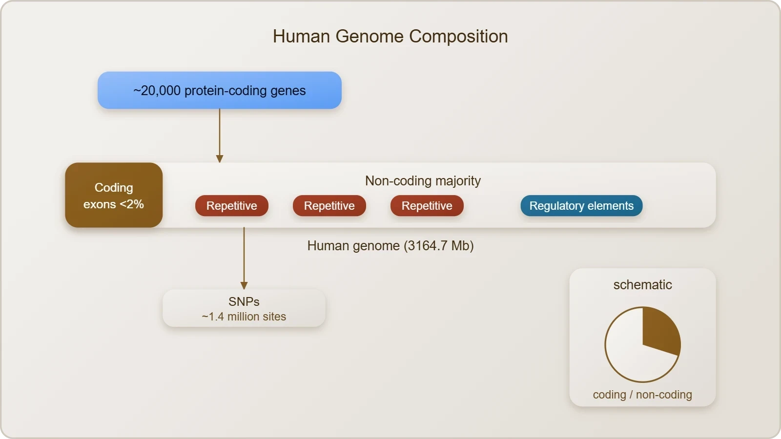
This lesson examines the salient features of the human genome as they emerged from that sequencing effort and traces what each finding implies for medicine, evolutionary biology, and the practice of research itself. The reference figures matter: 3164.7 million base pairs, an average gene of 3000 bases, a largest known gene (dystrophin) of 2.4 million bases, fewer than 2 per cent of the genome coding for proteins, and roughly 1.4 million single nucleotide polymorphisms catalogued. Each number carries a consequence, and each consequence has matured over two decades of post-genomic science.
Beyond the original findings, the story continues through the ENCODE project, genome-wide association studies, and the gradual refinement of the gene count to approximately 20,000 protein-coding genes. The genome's so-called dark matter, the vast non-coding majority once dismissed as junk, now occupies the centre of the field. Understanding why that shift occurred, and what it means for a student of molecular biology, is the purpose of the pages that follow.
On This Page
- The Architectural Surprises of the Sequenced Genome
- Repetitive DNA and the Grammar of the Genome
- Single Nucleotide Polymorphisms and the Logic of Variation
- The Dark Matter of the Genome and the ENCODE Correction
- Refining the Gene Count and the Post-Genomic Consensus
- Implications for Medicine and the Future of Genomics
- Common Misconceptions and Advanced Points
- Synthesis and the Road Ahead
The Architectural Surprises of the Sequenced Genome
The first complete read of the human genome produced a set of observations that read almost like a list of corrections to earlier textbooks. The genome contains 3164.7 million base pairs, distributed across 22 autosomes and the X and Y chromosomes, with chromosome 1 finishing last in May 2006. The average gene spans about 3000 bases, yet sizes vary enormously, and the largest known human gene, dystrophin, stretches across 2.4 million bases. These figures describe an architecture that is compact in places and extravagantly sprawling in others, a pattern that reflects the evolutionary pressures acting on different genomic regions.
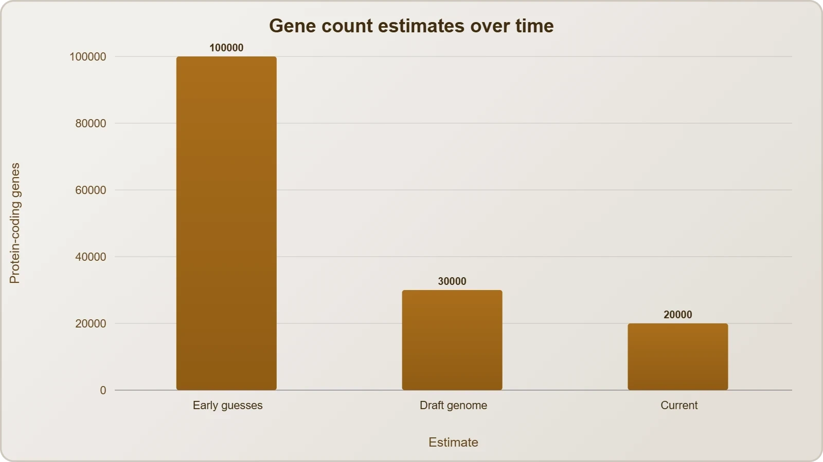
Perhaps the most consequential observation concerned gene number. The total was estimated at 30,000, dramatically lower than earlier guesses of 80,000 to 140,000. Equally striking, almost all nucleotide bases, 99.9 per cent, are exactly the same in all humans. The functions remain unknown for over 50 per cent of the discovered genes, a humbling admission that persists in updated form today. Together these findings suggested that human complexity arises less from the number of genes than from how those genes are regulated, spliced, and combined.
Gene Density and Chromosomal Inequality
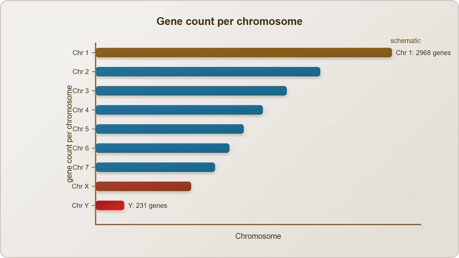
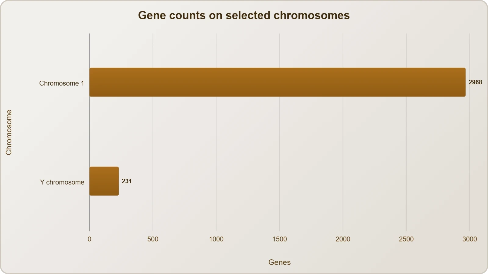
Genes are not distributed evenly across the chromosomes. Chromosome 1 carries the most genes, at 2968, while the Y chromosome carries the fewest, at 231. This asymmetry reflects both the small effective population size of the Y chromosome and its peculiar evolutionary history, including extensive repeat accumulation and a paucity of recombination along most of its length. Gene-dense regions tend to correlate with higher GC content and more open chromatin, while gene-poor regions often correspond to the lamina-associated domains that sit near the nuclear periphery.
The practical implication is that chromosomal location matters when interpreting variants. A pathogenic variant in a gene-dense region may affect neighbouring regulatory elements, while variants in gene deserts can act over long distances through chromatin looping. Modern clinical genomics therefore treats the linear sequence as only one layer of information, layering chromatin conformation, histone modification, and three-dimensional contact maps on top of the primary base order.
The Coding Fraction and Its Limits
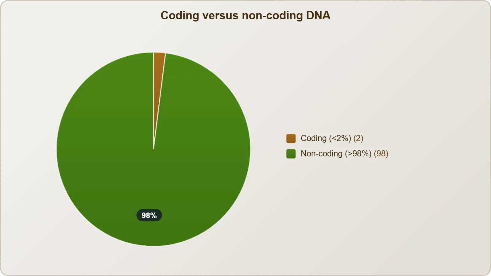
Less than 2 per cent of the genome codes for proteins, a figure that initially seemed to diminish the importance of the rest. That interpretation proved premature. The coding exons are indeed a small minority, but the transcripts they generate are embedded in a much larger network of regulatory sequence, non-coding RNA genes, and structural elements. The 2 per cent figure is best read as a statement about protein-coding capacity, not about functional importance.
Within that small fraction, alternative splicing multiplies the proteome far beyond the gene count. A single gene with twenty exons can generate hundreds of distinct transcripts through differential exon inclusion, and the human transcriptome contains well over 100,000 distinct mRNA species. This combinatorial logic explains how roughly 20,000 protein-coding genes can specify the staggering diversity of human cell types, tissues, and developmental stages.
Repetitive DNA and the Grammar of the Genome
Repeated sequences make up a very large portion of the human genome, and their abundance was one of the project's most unexpected findings. Repetitive sequences are stretches of DNA repeated many times, sometimes hundreds to thousands of times, and they are thought to have no direct coding function. Yet they shed light on chromosome structure, dynamics, and evolution, and they provide the polymorphism that underpins genetic mapping and forensic identification. Far from being inert filler, repeats shape how chromosomes fold, pair, and evolve.
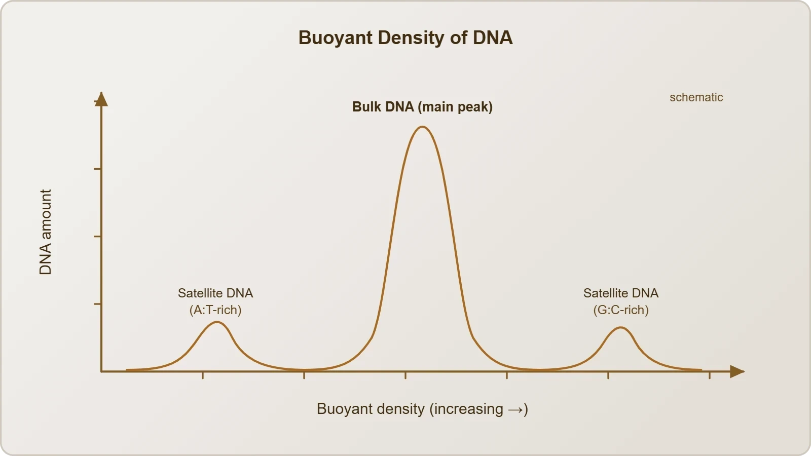
Repetitive DNA separates from bulk genomic DNA as distinct peaks during density gradient centrifugation. The bulk DNA forms a major peak, while the smaller satellite peaks correspond to satellite DNA. Depending on base composition (A:T rich or G:C rich), segment length, and the number of repetitive units, satellite DNA is classified into categories including microsatellites and minisatellites. Each class has its own mutation rate, its own chromosomal distribution, and its own utility in research and diagnostics.
Classes of Repetitive Elements
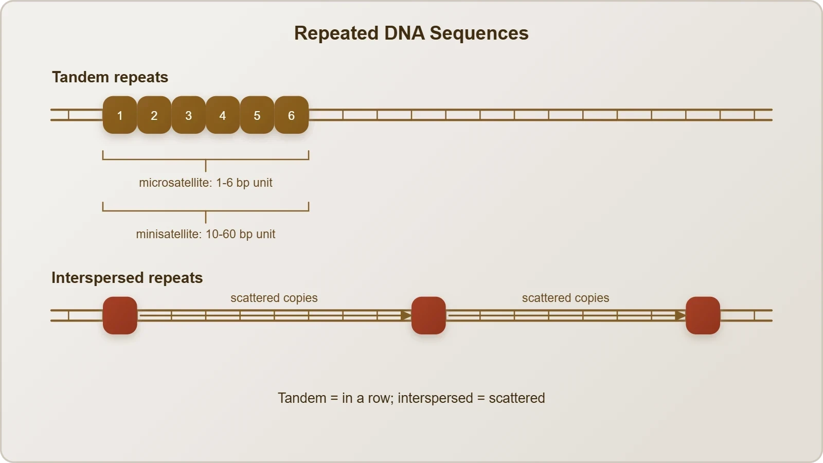
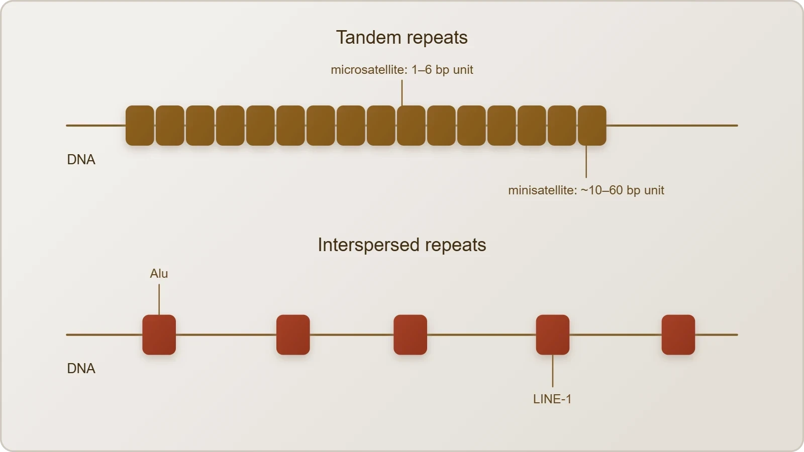
Tandem repeats, in which a short motif is arrayed head to tail, include microsatellites with repeat units of one to six bases and minisatellites with units of roughly ten to sixty bases. Interspersed repeats, by contrast, are dispersed copies of mobile elements such as Alu sequences and LINE-1 retrotransposons, which together account for a substantial share of the genome. These elements can create new splice sites, donate regulatory motifs, and occasionally disrupt genes, and their activity has shaped mammalian evolution profoundly.
The distinction matters clinically. Expansion of a trinucleotide repeat underlies Huntington disease and several spinocerebellar ataxias, where the number of CAG units crosses a pathogenic threshold. Microsatellite instability, arising from defective mismatch repair, is a hallmark of Lynch syndrome and a predictive biomarker for immunotherapy response. Repetitive DNA is therefore both a structural feature of the genome and a direct source of human disease.
Why Repeats Reveal Evolutionary History
Because repetitive elements accumulate mutations relatively freely, they serve as molecular clocks. Comparing Alu insertion sites between species allows researchers to date divergence events and reconstruct phylogenies with remarkable precision. Within populations, the copy number of specific repeats varies between individuals, generating the polymorphism that makes these loci informative for ancestry inference and forensic matching.
The evolutionary perspective also explains why repeats persist despite occasional harm. Most insertions occur in non-coding regions where they have little immediate effect on reproductive fitness, so they drift through populations and accumulate generation after generation. This accumulation is one of the foundations of genomic variability, and it illustrates a broader principle: much of genome evolution proceeds through neutral or nearly neutral change rather than through adaptive selection alone.
Single Nucleotide Polymorphisms and the Logic of Variation
Scientists have identified about 1.4 million locations where single-base DNA differences occur in humans, known as single nucleotide polymorphisms, or SNPs and pronounced snips. This information promised to revolutionise the process of finding chromosomal locations for disease-associated sequences and tracing human history. The promise has been substantially realised. Modern reference panels now catalogue tens of millions of SNPs, and imputation from these panels allows researchers to interrogate variants that were never directly genotyped in a study cohort.
Polymorphism, variation at the genetic level, arises due to mutations. New mutations may appear in somatic cells or in germ cells, and only germ-cell mutations that do not seriously impair the ability to produce offspring can spread through a population via sexual reproduction. Allelic sequence variation is traditionally described as DNA polymorphism when more than one variant at a locus occurs in the human population with a frequency greater than 0.01. In simple terms, an inheritable mutation observed at high frequency is a polymorphism.
From Polymorphism to Genome-Wide Association Studies
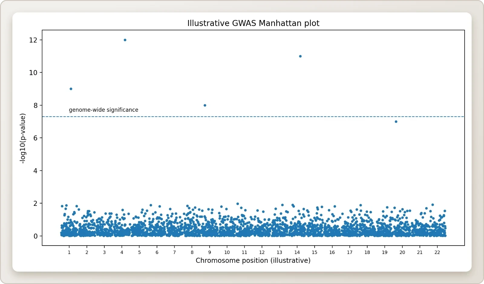
Genome-wide association studies, or GWAS, exploit the density of SNPs to link genomic regions to traits and diseases. The logic rests on linkage disequilibrium: nearby variants are inherited together more often than expected by chance, so a genotyped SNP can serve as a proxy for an untyped causal variant. By comparing allele frequencies between cases and controls across hundreds of thousands of markers, GWAS identifies loci associated with conditions such as type 2 diabetes, Crohn disease, and age-related macular degeneration.
The statistical foundation is straightforward. For each SNP, a chi-square or logistic regression test compares genotype distributions, and the resulting p-values are corrected for the enormous number of tests performed. A conventional genome-wide significance threshold of ##p < 5 \times 10^{-8}## controls the family-wise error rate at approximately 0.05 across roughly one million independent tests. The effect sizes recovered are typically modest, with odds ratios often between 1.1 and 1.5, which is why polygenic risk scores aggregate thousands of small contributions rather than relying on single markers.
Interpreting Effect Sizes and Heritability
Most GWAS hits fall in non-coding regions, reinforcing the lesson that regulatory variation dominates common disease risk. The gap between the heritability estimated from twin studies and the variance explained by significant SNPs, sometimes called missing heritability, has narrowed as sample sizes have grown and as rare variants, structural variants, and gene-gene interactions have entered the analysis. The current consensus treats common disease as highly polygenic, with contributions spread across thousands of loci of small effect.
For students, the practical lesson is that a statistically significant association is not a mechanism. Follow-up work requires fine-mapping, functional assays, and often chromatin interaction data to connect a variant to a target gene. The SNP is a signpost, not a destination, and the interpretive work of post-GWAS biology is where most of the intellectual effort now lies.
The Dark Matter of the Genome and the ENCODE Correction
The finding that less than 2 per cent of the genome codes for proteins led many to describe the remainder as junk DNA. That label has not aged well. The ENCODE project, launched as a follow-up to the Human Genome Project, set out to map functional elements across the genome, including transcribed regions, transcription factor binding sites, chromatin states, and histone modifications. Its 2012 publications reported that a large majority of the genome shows at least one biochemical signature of activity in at least one cell type.
The interpretation of that figure remains contested. Critics note that biochemical activity is not the same as evolutionary conservation or functional necessity, and that a substantial fraction of the genome is likely to be neutral. The balanced view, now widely accepted, is that the non-coding majority contains a dense mixture of regulatory elements, non-coding RNA genes, structural sequences, and genuinely dispensable material. The genome's dark matter is neither uniformly functional nor uniformly junk; it is a heterogeneous landscape that requires cell-type-specific maps to interpret.
What ENCODE Actually Demonstrated
ENCODE produced reference maps of DNase I hypersensitivity, histone modifications such as H3K4me3 and H3K27ac, and transcription factor occupancy across dozens of human cell types. These maps revealed that enhancers and promoters are far more numerous than genes, that many are active only in specific developmental windows, and that disease-associated variants from GWAS are strongly enriched within them. The project thereby supplied the functional annotation that the original genome sequence lacked.
The practical consequence is that interpreting a patient's variant now requires knowing which regulatory element it disrupts and in which tissue. A variant in an enhancer active only in pancreatic beta cells may be invisible in a blood sample yet decisive for diabetes risk. This tissue-specific logic has driven the growth of single-cell epigenomics and has made chromatin data an essential companion to sequence data in clinical interpretation.
Non-Coding RNAs as Functional Elements
Among the functional non-coding elements are thousands of long non-coding RNAs, microRNAs, and circular RNAs. MicroRNAs regulate mRNA stability and translation, and their dysregulation is implicated in cancer and cardiovascular disease. Long non-coding RNAs such as XIST orchestrate chromosome-wide silencing, while others act as scaffolds for chromatin-modifying complexes. These molecules demonstrate that the genome's regulatory capacity extends well beyond protein-coding sequence.
The discovery of CRISPR systems, themselves bacterial adaptive immune elements, illustrates how studying non-coding and repetitive biology yields transformative technology. The same logic applies to RNA interference, telomerase, and the spliceosome, all of which emerged from investigations of sequences once considered peripheral. The lesson for students is that dismissing uncharacterised sequence as unimportant has repeatedly proven costly.
Refining the Gene Count and the Post-Genomic Consensus
The original estimate of 30,000 genes has since been refined to approximately 20,000 protein-coding genes, a figure that places humans closer to nematodes than to the earlier expectations of complexity. The refinement came from improved annotation, comparative genomics, and the recognition that many predicted open reading frames are not translated. The current consensus, maintained by reference databases such as GENCODE, lists roughly 19,900 protein-coding genes alongside tens of thousands of non-coding RNA genes.
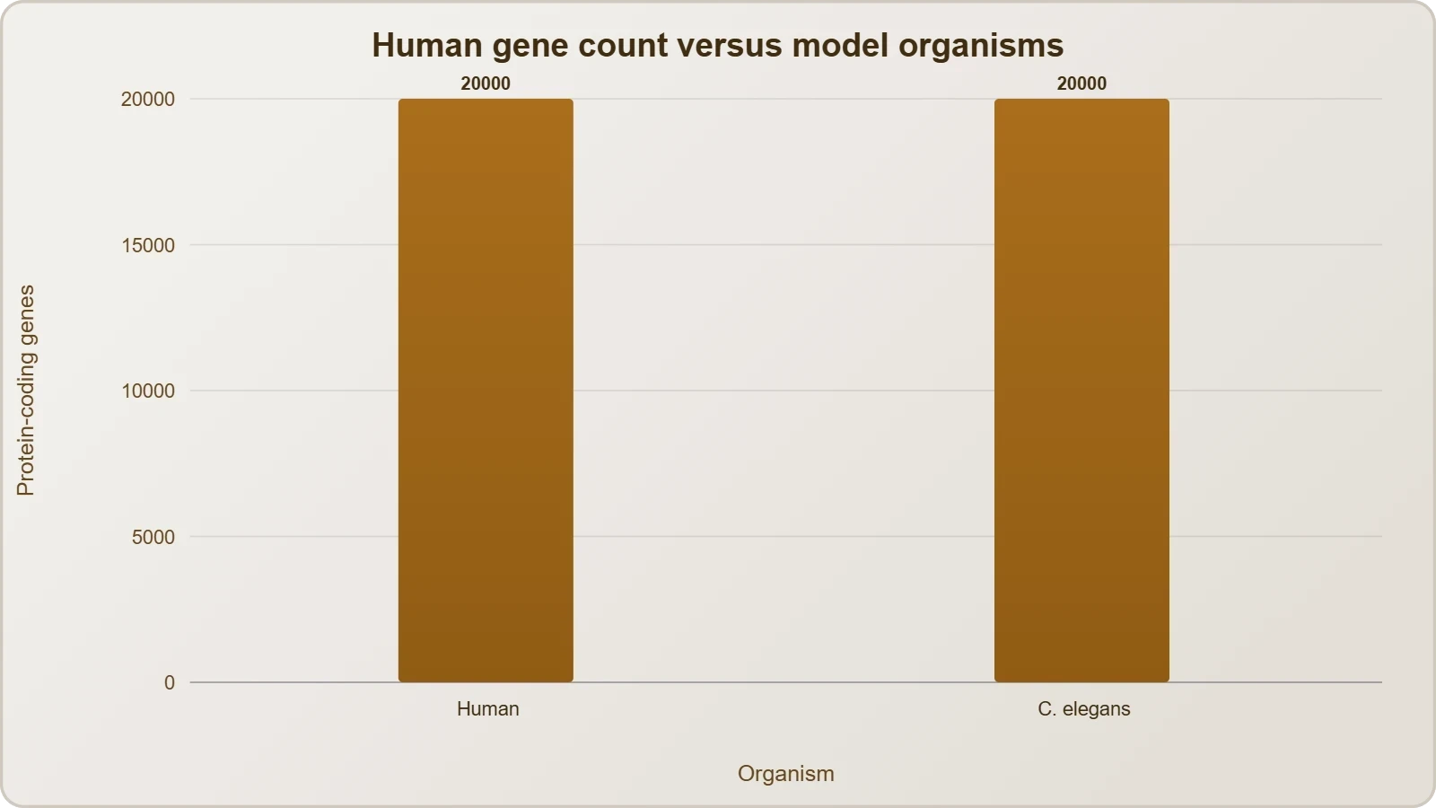
This downward revision reinforced a conceptual shift. Human complexity is not encoded in gene number but in regulatory architecture, alternative splicing, and the combinatorial assembly of protein complexes. The same gene can produce different isoforms in different tissues, and the same genome can generate hundreds of cell types through differential expression. Gene count, in other words, is a poor proxy for biological sophistication.
Comparative Genomics and Model Organisms
Sequencing non-human organisms has been integral to interpreting the human genome. Bacteria, yeast, Caenorhabditis elegans, Drosophila, rice, and Arabidopsis have all been sequenced, and each provides a reference point for identifying conserved elements and reconstructing evolutionary relationships. Model organisms allow experimental manipulation that would be impossible in humans, and their genomes illuminate which features are ancient and which are lineage-specific.
Comparative analysis reveals that roughly 60 per cent of human genes have identifiable homologues in Drosophila and that core cellular machinery is conserved across billions of years. At the same time, human-specific regulatory innovations, including expanded enhancer repertoires in the neocortex, distinguish our lineage. The synthesis of conservation and divergence is what makes comparative genomics so powerful for understanding human biology.
From Sequence to Systems
The greatest impact of the human genome sequence may be the shift from studying one or a few genes at a time to interrogating whole systems. High-throughput technologies now allow researchers to examine all transcripts in a tissue, all proteins in a tumour, or the interconnected networks through which tens of thousands of genes orchestrate the chemistry of life. This systems perspective defines contemporary molecular biology and underpins precision medicine.
Deriving meaningful knowledge from DNA sequences will define research through the coming decades. The task requires expertise and creativity from tens of thousands of scientists across disciplines in both public and private sectors worldwide. The genome is a starting point, not an endpoint, and the interpretive work of functional genomics, proteomics, and computational biology is where the next generation of discoveries will be made.
Implications for Medicine and the Future of Genomics
The clinical implications of the genome project have unfolded more slowly than the initial optimism suggested, but they are now substantial. Pharmacogenomics uses variants in genes such as CYP2D6 and TPMT to guide drug dosing, reducing adverse reactions. Cancer genomics matches targeted therapies to driver mutations in tumours, and liquid biopsies detect circulating tumour DNA for early recurrence monitoring. Rare disease diagnosis through exome and genome sequencing now yields a molecular answer in roughly a third of previously undiagnosed cases.
Polygenic risk scores aggregate thousands of common variants to estimate susceptibility to conditions such as coronary artery disease and type 2 diabetes. Their clinical utility depends on ancestry representation, since most discovery cohorts have been of European descent, and on calibration across populations. Equity in genomic medicine is therefore both a scientific and an ethical priority, and the field is actively working to diversify reference panels and biobanks.
Pharmacogenomics and Precision Therapeutics
Genetic variation influences drug metabolism, transport, and target sensitivity. Variants in CYP2C19 affect clopidogrel activation, and genotyping now guides antiplatelet therapy after coronary stenting. HLA-B*57:01 screening prevents abacavir hypersensitivity, and TPMT genotyping prevents thiopurine toxicity in leukaemia treatment. These examples show that the genome's practical value often lies in avoiding harm rather than in predicting destiny.
The computational infrastructure behind these applications is substantial. Variant calling pipelines process billions of sequencing reads, and annotation tools cross-reference databases of known pathogenic variants. A simplified illustration of the logic used to filter variants by allele frequency appears below, capturing the kind of reasoning that clinical bioinformaticians apply routinely.
variants = [
    {"rsid": "rs6025", "gene": "F5", "af": 0.02, "impact": "pathogenic"},
    {"rsid": "rs429358", "gene": "APOE", "af": 0.15, "impact": "risk_factor"},
    {"rsid": "rs334", "gene": "HBB", "af": 0.01, "impact": "pathogenic"},
]

rare_pathogenic = [
    v for v in variants
    if v["af"] < 0.05 and v["impact"] == "pathogenic"
]

for v in rare_pathogenic:
    print(f"{v['rsid']} in {v['gene']} (AF={v['af']})")
Ethical Boundaries and Data Governance
Genomic data are uniquely identifying and inherently familial, which creates governance challenges that ordinary medical data do not present. A proband's sequence reveals information about relatives who never consented to testing, and re-identification from supposedly anonymised data has been demonstrated repeatedly. Genetic discrimination in insurance and employment remains a live concern, addressed in some jurisdictions by legislation such as the Genetic Information Nondiscrimination Act in the United States.
Balancing open data sharing against privacy requires tiered access models, consent frameworks that anticipate secondary use, and robust de-identification standards. The research community has largely converged on controlled-access repositories for individual-level data while releasing aggregate statistics openly. These arrangements are imperfect but represent a workable compromise between the scientific value of sharing and the legitimate claims of individuals whose genomes are at stake.
Common Misconceptions and Advanced Points
Several misconceptions persist about the human genome, and correcting them sharpens understanding. The claim that humans have fewer genes than a grape or a nematode is often overstated; the comparison depends on which annotation is used and ignores non-coding genes entirely. The assertion that 98 per cent of the genome is junk misreads the coding fraction as a functional fraction. And the idea that a single gene determines a single trait collapses under the weight of pleiotropy, epistasis, and environmental interaction.
Another frequent error concerns the 99.9 per cent identity figure. That number refers to single nucleotide differences in aligned regions and excludes insertions, deletions, and structural variants, which contribute additional variation. Two genomes differ by roughly three million SNPs plus several thousand structural changes, and the functional consequences of those differences are highly context-dependent. Precision in stating what the figure measures prevents overconfident conclusions about human similarity.
Pleiotropy, Penetrance, and Context
A single gene often influences multiple traits, a phenomenon called pleiotropy. Variants in the fibrillin gene cause Marfan syndrome with skeletal, ocular, and cardiovascular features, illustrating how one locus can affect several organ systems. Penetrance describes the probability that a genotype produces the phenotype, and it varies with age, environment, and modifier genes. These concepts explain why genetic testing results require careful counselling rather than deterministic interpretation.
Epistasis, the interaction between genes, further complicates prediction. Two variants that are individually benign may combine to produce disease, and a protective variant at one locus may buffer a risk variant at another. Modelling these interactions requires large sample sizes and sophisticated statistical methods, and it remains one of the frontier challenges of computational genetics.
Structural Variation and the Invisible Genome
Beyond SNPs lie copy number variants, inversions, and translocations that can span millions of bases. Short-read sequencing often misses these events, and long-read technologies have revealed that structural variation is far more common than once assumed. Some structural variants are benign polymorphisms, while others disrupt genes or regulatory elements and cause disease. Incorporating them into clinical analysis is an active area of development.
The pangenome reference, which incorporates diverse human assemblies rather than a single linear sequence, addresses the bias inherent in earlier references. By representing variation directly, it improves alignment accuracy in regions that differ between populations. This shift from a single reference to a graph-based representation marks a significant methodological advance and promises more equitable genomic medicine.
Synthesis and the Road Ahead
The salient features of the human genome, taken together, describe a system that is compact in coding capacity, expansive in regulation, and rich in variation. The 3164.7 million base pairs, the 30,000-gene estimate later refined to about 20,000, the sub-2 per cent coding fraction, the abundant repeats, and the 1.4 million SNPs each contribute to a coherent picture. That picture is of a genome whose complexity lies in organisation and control rather than in raw gene count, and whose variation provides both the substrate for evolution and the toolkit for identification.
The implications extend across medicine, evolutionary biology, and forensic science. GWAS and polygenic scores translate variation into risk estimates, pharmacogenomics translates it into prescribing decisions, and DNA fingerprinting translates it into identity. The ENCODE project and the study of non-coding RNAs have shown that the dark matter of the genome is functionally consequential, while the pangenome reference is correcting the biases of a single linear standard. Each of these developments builds on the original findings rather than replacing them.
The next lesson turns to DNA fingerprinting, where the polymorphism described here becomes a practical instrument for identification. The principles established in this lesson, particularly the distinction between coding and non-coding variation and the inheritance of polymorphic repeats, provide the conceptual foundation for that technique. Mastery of these ideas prepares the learner to appreciate both the power and the limitations of forensic genetics, and to evaluate claims about what a genome can and cannot reveal.
Also Read
- No links available.
From our network :
- How to Print Cheaply: Cutting the Cost per PageA practical, measured guide to lowering what each printed page costs — duplex and draft modes, third-party ink, yield mathematics, and knowing when a new printer beats refills.
- 10 Physics Numerical Problems with Solutions for IIT JEEPrepare for IIT JEE with 10 physics numerical problems, complete with detailed solutions and conceptual explanations. Ideal for mastering kinematics, thermodynamics, electromagnetism, and optics.
- 98% of Global MBA Programs Now Prefer GRE Over GMAT Focus EditionExplore why 98% of global MBA programs now prefer the GRE over GMAT Focus. Learn about the shorter GRE format, verbal logic importance, and strategic versatility for students.
- Trump Political Strategy How Geopolitical Stunts Serve As Media Diversions
- Do You Need a New Router or Is Your Internet Plan the Problem?A practical comparison of the signs that point to router limits versus signs your broadband speed or provider is the bottleneck, so you can decide what to replace before spending money.
- EV 2.0: The Solid-State Battery Breakthrough and Global Factory ExpansionDiscover the impact of the Solid-State Battery Breakthrough on the EV market. Learn about CATL and BYD stock growth, global factory expansion in Europe, and the future of EV 2.0 technology.
- AI-Powered 'Precision Diagnostic' Replaces Standard GRE Score ReportsDiscover the new GRE Precision Diagnostic. Learn how AI-powered behavioral analytics and time-to-solve tracking are replacing standard GRE score reports to empower students.
- Where to Put Your Wireless Router for Better CoverageA practical, physics-grounded guide to router placement: why the centre of the home beats the corner, how walls and metal sap signal, and how to run a simple survey that proves the improvement.
- Analyzing Trump Deportation Numbers Insights Into The 2026 Immigration Crackdown
RESOURCES
- Resources will be updated soon.