Ecology becomes a genuinely predictive science only when its central processes can be counted, compared, and modelled. A forest, a lake, and a grassland may all appear green and vigorous, yet their actual rates of carbon capture, litter breakdown, and energy transfer differ by orders of magnitude. Quantitative ecology supplies the instruments and arithmetic that convert these impressions into defensible numbers: grams of dry matter per square metre per year, kilocalories moving between trophic levels, and half-lives of leaf litter on a forest floor. This lesson builds directly on the discussion of ecosystem services and human dependence, asking a sharper question — how do we actually measure the flows that underpin those services?
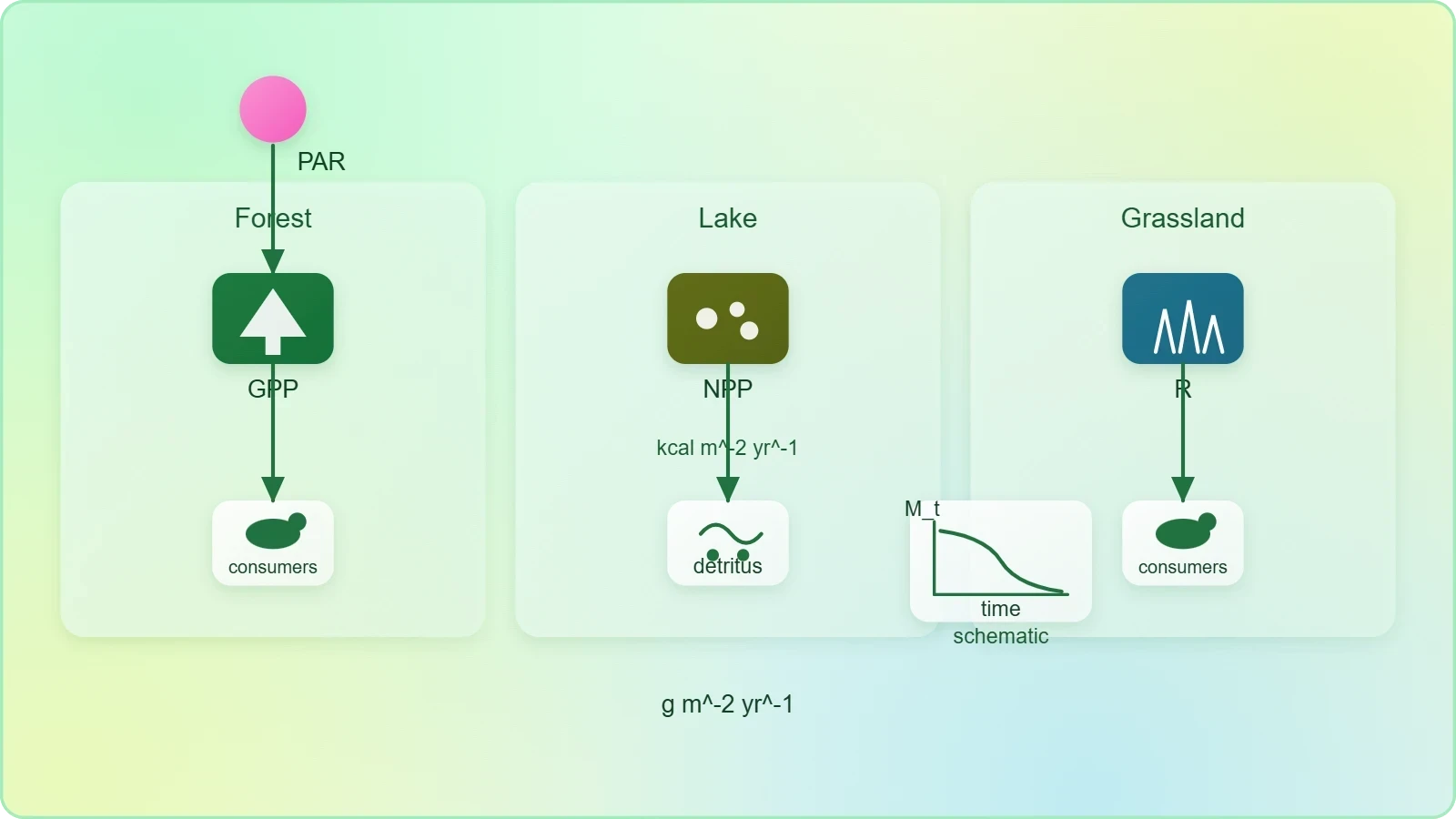
The analytical toolkit assembled here spans field biology, chemistry, and statistics. We will derive gross and net primary productivity from first principles, walk through the light–dark bottle technique used in aquatic systems, examine how stable isotopes trace carbon and nitrogen through food webs, and apply inferential statistics to compare sites. A landmark case study, the Hubbard Brook Experimental Forest, demonstrates how long-term quantitative monitoring revealed the hidden costs of deforestation. Throughout, the emphasis falls on disciplined measurement: correct units, honest error bars, and cautious interpretation of ecological pyramids that are often drawn more confidently than the underlying data justify.
By the close of the lesson, you should be able to compute ecological efficiency from raw productivity figures, diagnose why oceanic productivity lags far behind its vast area, and recognise the unit-conversion traps that quietly corrupt published datasets. These skills prepare the ground for the next lesson on stability, disturbance, and succession, where quantitative baselines become essential for judging whether an ecosystem is recovering, degrading, or simply fluctuating within normal bounds.
On This Page
- Productivity as a Measurable Rate: GPP, NPP, and Respiration
- Measuring Aquatic Productivity: The Light–Dark Bottle Method
- Decomposition as a Quantifiable Process
- Energy Flow, Trophic Levels, and Ecological Pyramids
- Common Errors in Units, Conversions, and Data Interpretation
- From Measurement to Model: Integrating the Quantitative Picture
Productivity as a Measurable Rate: GPP, NPP, and Respiration
Primary productivity is the rate at which biomass or organic matter is produced per unit area over a period of time by plants during photosynthesis. It is expressed either as weight, typically grams per square metre, or as energy, typically kilocalories per square metre. Because a single harvest tells you only a standing crop, the rate of biomass production — productivity — must be expressed per unit time, such as ##\text{g m}^{-2}\text{ yr}^{-1}## or ##(\text{kcal m}^{-2})\text{ yr}^{-1}##, so that ecosystems of different types can be compared fairly. Confusing a standing biomass with a productivity rate remains one of the most frequent errors in student reports.
Gross primary productivity (GPP) is the rate of production of organic matter during photosynthesis, while a considerable portion of that fixed carbon is immediately consumed by the plants themselves in respiration. Subtracting respiration losses (R) from GPP yields net primary productivity (NPP), the biomass actually available for consumption by heterotrophs — herbivores and decomposers alike. Secondary productivity, by contrast, is the rate at which consumers form new organic matter. Primary productivity depends on plant species, nutrient availability, environmental conditions, and photosynthetic capacity, which is why it varies so widely between ecosystems.
Worked Calculations for GPP, NPP, and Efficiency
Consider a temperate meadow where enclosure measurements show a GPP of ##2200\ \text{g m}^{-2}\text{ yr}^{-1}## and plant respiration of ##900\ \text{g m}^{-2}\text{ yr}^{-1}##. Applying the fundamental relationship gives the net figure directly:
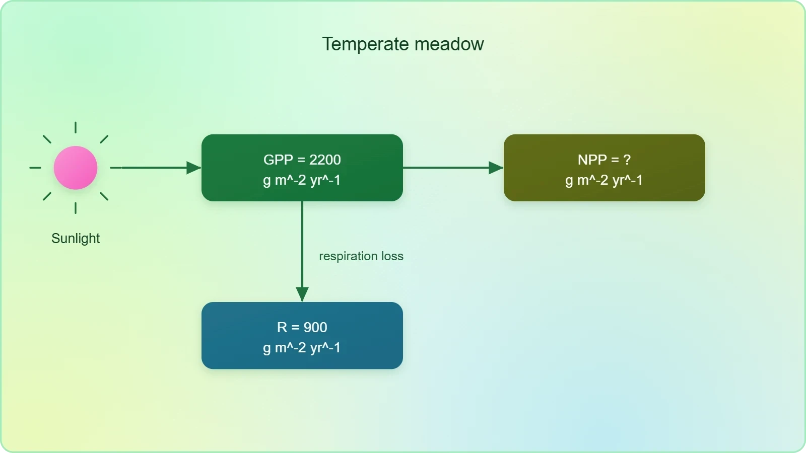
If herbivores in that meadow consume ##260\ \text{g m}^{-2}\text{ yr}^{-1}## of plant material, the consumption efficiency is ##260/1300 \approx 20\%##, a plausible figure for grassland systems. Suppose the herbivores assimilate 60% of ingested energy and respire the remainder; their net secondary production then becomes ##260 \times 0.60 \times 0.40 \approx 62\ \text{g m}^{-2}\text{ yr}^{-1}##. Chaining these ratios produces the ecological (Lindeman) efficiency, the fraction of energy at one trophic level transferred to the next, typically around 10% and rarely exceeding 20% in natural systems.
A second example illustrates energy units. If a producer level fixes ##20{,}000\ \text{kcal m}^{-2}\text{ yr}^{-1}## and the primary consumers assimilate ##2{,}000\ \text{kcal m}^{-2}\text{ yr}^{-1}##, the transfer efficiency is exactly 10%. Students should always verify dimensional consistency: dividing kilocalories by kilocalories yields a dimensionless ratio, whereas dividing grams by kilocalories produces a meaningless number. Writing units at every intermediate step, rather than only in the final answer, catches most arithmetic slips before they propagate into conclusions about ecosystem function.
Global Patterns and the Ocean Paradox
The annual net primary productivity of the whole biosphere is approximately 170 billion tons of organic matter on a dry-weight basis. Of this total, the oceans contribute only about 55 billion tons despite covering roughly 70% of Earth's surface, leaving the remainder — well over 100 billion tons — to land. The main reason for this disparity is the scarcity of nutrients, particularly nitrogen and phosphorus, in the sunlit surface waters of the open ocean, compounded by the fact that light attenuates rapidly with depth, restricting photosynthesis to a thin photic zone. Coastal upwellings, where nutrient-rich deep water rises, are the striking exception.
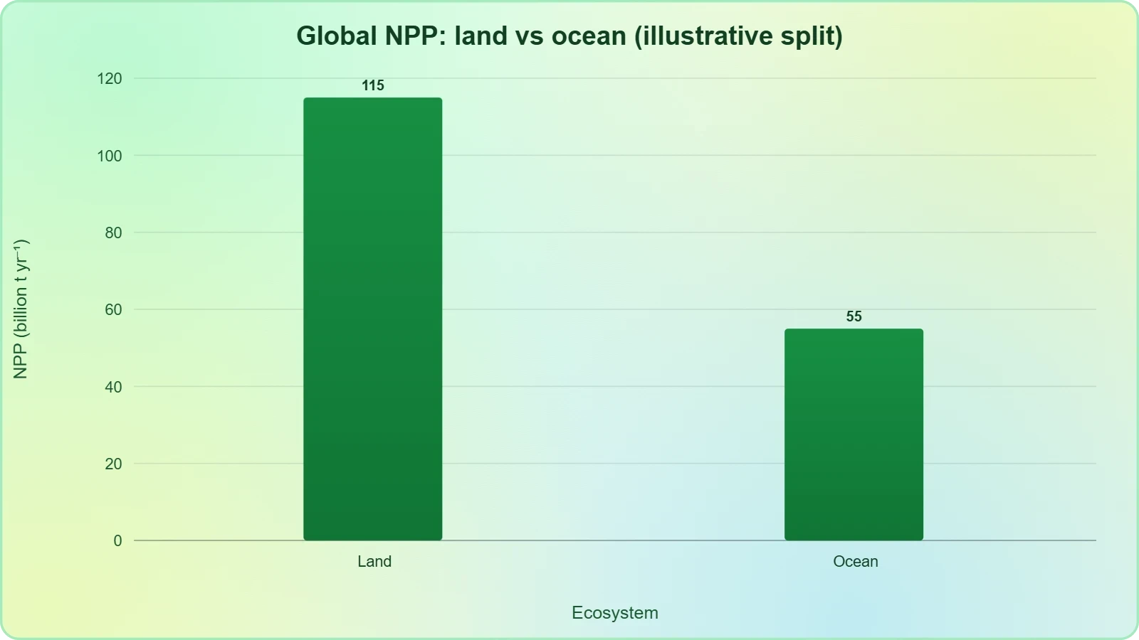
This asymmetry carries practical weight. Terrestrial ecosystems, with their deeper soils and denser nutrient reservoirs, respond to added nutrients with measurable productivity gains, while open-ocean fertilisation experiments produce modest and often transient responses. When interpreting global productivity maps, remember that area alone predicts very little; nutrient supply, temperature, and water availability jointly govern the rate. The ocean paradox also explains why marine food webs concentrate biomass in relatively few productive regions and why fisheries depend disproportionately on narrow upwelling zones.
Measuring Aquatic Productivity: The Light–Dark Bottle Method
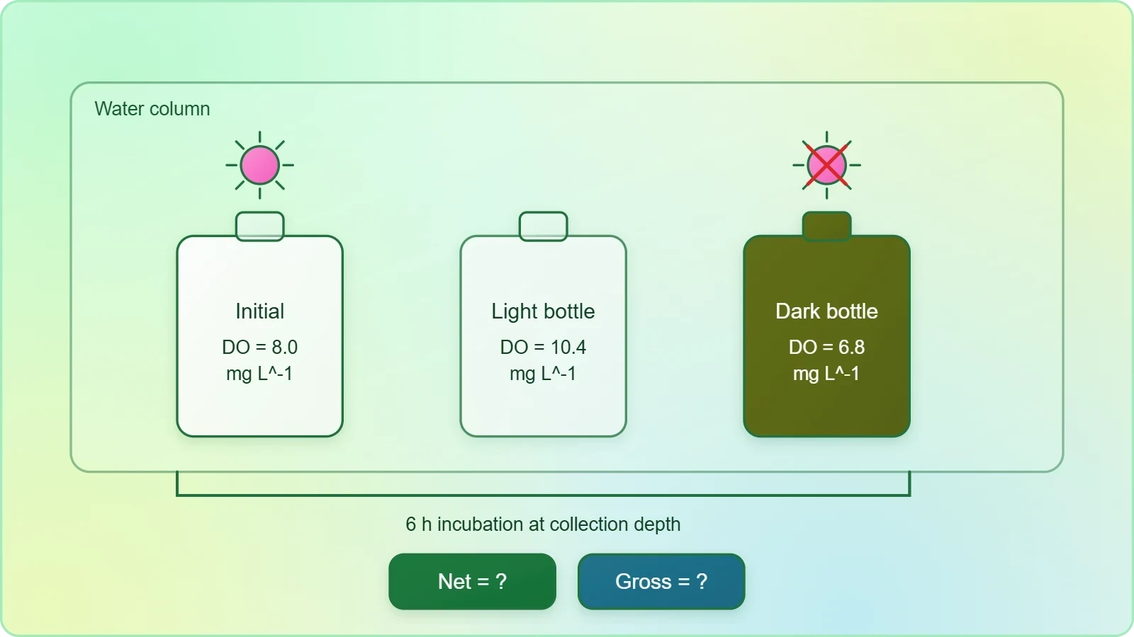
Terrestrial productivity can be estimated by harvesting quadrats, but aquatic systems demand a different approach because phytoplankton cannot be clipped and weighed conveniently. The light–dark bottle method exploits the oxygen balance of enclosed water samples. Water is collected at a known depth, sealed into paired transparent and opaque bottles, and incubated in situ at the collection depth for a fixed period. The transparent bottle permits photosynthesis and respiration; the opaque bottle permits only respiration. Comparing dissolved oxygen before and after incubation separates the two processes arithmetically.
The calculation follows a clean logic. If the light bottle gains oxygen relative to the initial reading, that gain represents net production; if the dark bottle loses oxygen, that loss represents respiration. Gross production is the sum of the two. Because oxygen and carbon are linked by the photosynthetic quotient, oxygen changes convert to carbon fixation using a standard factor, commonly around 1.2 grams of carbon per gram of oxygen evolved, though the exact ratio depends on the biochemical composition of the algae.
Interpreting Bottle Data and Its Limitations
Suppose an initial sample reads ##8.0\ \text{mg L}^{-1}## dissolved oxygen, the light bottle after six hours reads ##10.4\ \text{mg L}^{-1}##, and the dark bottle reads ##6.8\ \text{mg L}^{-1}##. Net production is ##10.4 - 8.0 = 2.4\ \text{mg L}^{-1}## of oxygen, respiration is ##8.0 - 6.8 = 1.2\ \text{mg L}^{-1}##, and gross production is ##2.4 + 1.2 = 3.6\ \text{mg L}^{-1}## over the incubation. Scaling to a daily rate requires care: a six-hour incubation cannot simply be multiplied by four unless light conditions are representative, so most protocols incubate for a full diel cycle or apply a light-response correction.
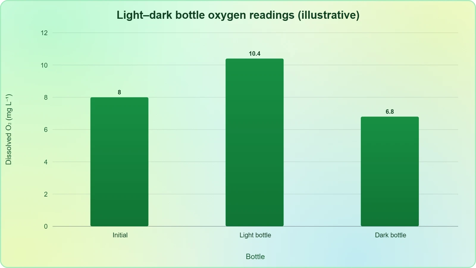
The method has well-known artefacts. Bottle enclosure excludes mixing and grazing by larger zooplankton, can cause photoinhibition in the confined volume, and may alter dissolved gas exchange with the atmosphere. Results therefore represent a conservative estimate of true water-column productivity. Modern practice often pairs bottle incubations with fluorometric or oxygen-sensor measurements to cross-validate, and researchers report incubation duration, depth, and conversion factors explicitly so that datasets remain comparable across studies and laboratories.
Stable Isotopes as Tracers of Energy Flow
Stable isotope analysis has transformed the study of energy flow because it integrates feeding over weeks or months rather than capturing a single meal. Carbon isotope ratios (##\delta^{13}\text{C}##) distinguish, for example, C3 from C4 plants and pelagic from benthic carbon sources, while nitrogen ratios (##\delta^{15}\text{N}##) increase by roughly 3 to 4 parts per thousand with each trophic step, providing a continuous index of trophic position. A consumer's nitrogen signature therefore estimates how high it feeds in the web without direct observation of feeding.
Applications range from identifying the nursery habitats of juvenile fish to quantifying how much terrestrial carbon enters stream food webs. The technique requires careful baseline correction, because the isotopic signature of the primary producers at the base of the web varies by location and season. Mixing models, increasingly Bayesian in formulation, estimate the proportional contributions of multiple sources to a consumer's diet. When combined with productivity measurements, isotope data reveal not only who eats whom but how much energy actually moves along each pathway.
Decomposition as a Quantifiable Process
Decomposers break down complex organic matter into inorganic substances such as carbon dioxide, water, and nutrients, and this process is called decomposition. Dead plant remains — leaves, bark, flowers — together with animal remains and fecal matter constitute detritus, the raw material for the process. The important steps are fragmentation, leaching, catabolism, humification, and mineralisation, and crucially these steps operate simultaneously on the detritus rather than in strict sequence. Detritivores such as earthworms fragment detritus into smaller particles, while leaching carries water-soluble inorganic nutrients down into the soil horizon where they may precipitate as unavailable salts.
Bacterial and fungal enzymes degrade detritus into simpler inorganic substances through catabolism. Humification then accumulates a dark, amorphous, colloidal substance called humus, highly resistant to microbial action and decomposing at an extremely slow rate, which serves as a reservoir of nutrients. Mineralisation releases inorganic nutrients from humus through further microbial degradation. Decomposition is largely an oxygen-requiring process, and its rate is governed by the chemical composition of the detritus and by climatic factors, especially temperature and soil moisture.
Litter Bags, Decay Constants, and Controlling Factors
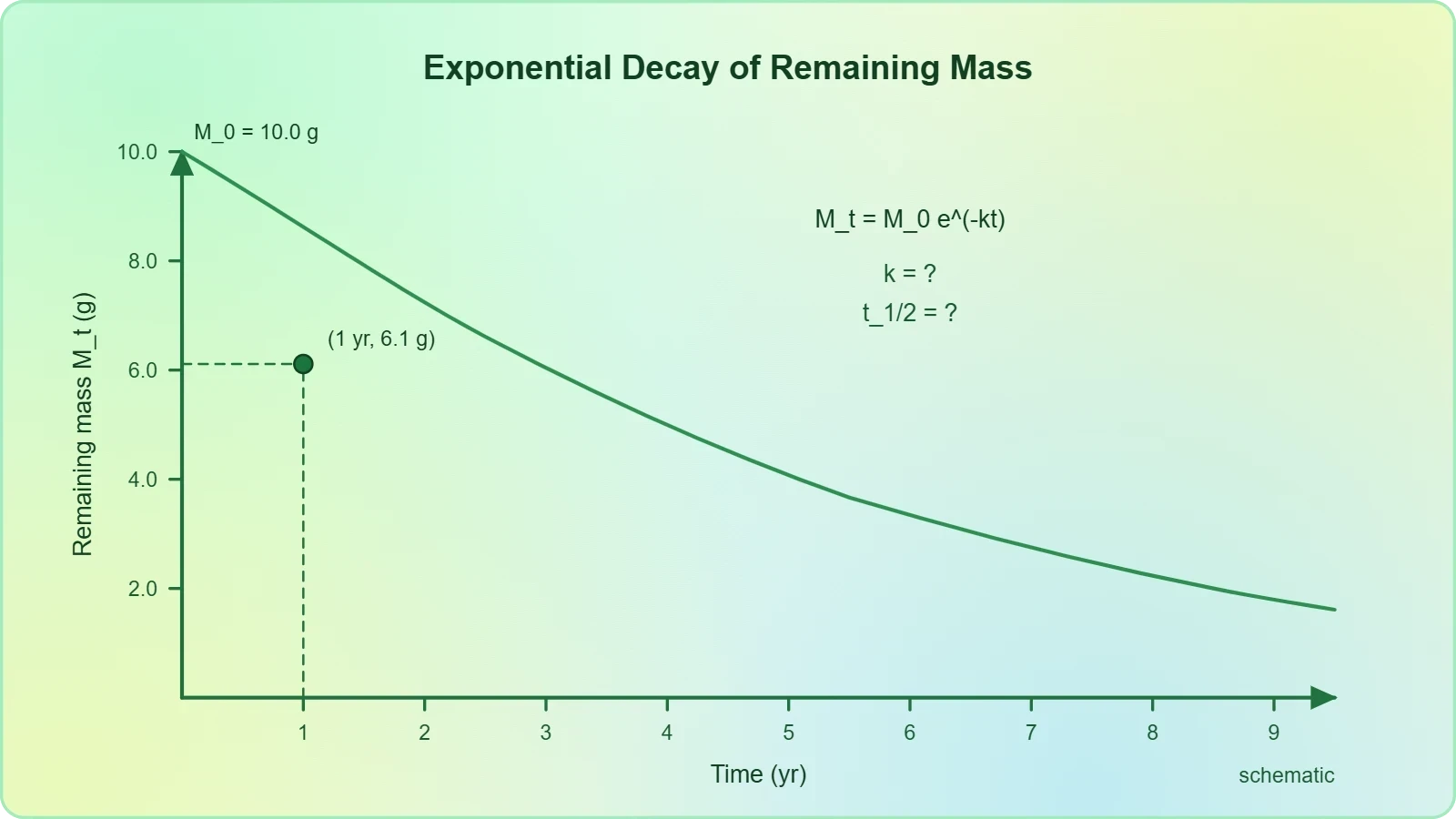
Quantitative decomposition studies typically use litter bags: known masses of dried leaf material sealed in mesh bags, buried or pinned to the soil surface, and retrieved at intervals. The remaining mass is plotted against time and fitted to a negative exponential model, where the decay constant ##k## summarises the rate:
If a litter bag starts at 10.0 g and retains 6.1 g after one year, then ##k = -\ln(0.61) \approx 0.49\ \text{yr}^{-1}##, implying a half-life of ##\ln 2 / k \approx 1.4## years. In a particular climatic condition, decomposition is slower when detritus is rich in lignin and chitin and quicker when it is rich in nitrogen and water-soluble substances such as sugars. Warm, moist environments favour decomposition, whereas low temperature and anaerobiosis inhibit it, causing organic material to accumulate.
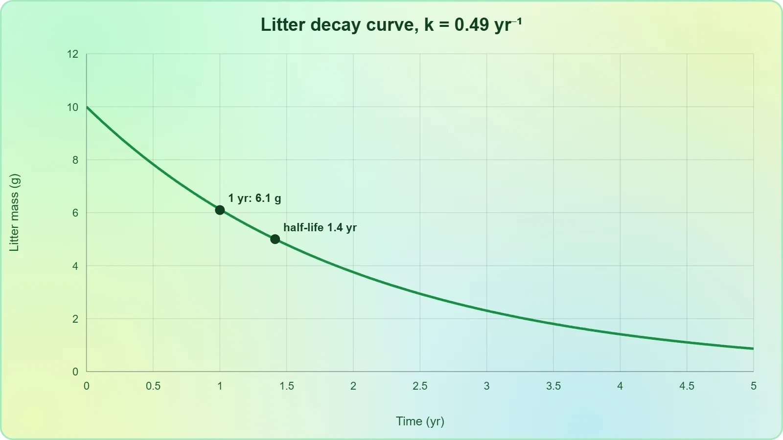
This explains the deep peat deposits of cold, waterlogged regions and the rapid litter disappearance in tropical forests. Comparing decay constants across sites therefore provides a quantitative index of both climate and litter quality, and repeated litter-bag experiments have become a standard tool for detecting shifts in decomposition associated with warming or nitrogen deposition. Students should record mesh size, initial moisture, and retrieval intervals, since these methodological details strongly influence the fitted decay constant and its comparability.
Statistical Comparison of Productivity Across Sites
Comparing productivity between sites requires more than ranking two averages. Replicate quadrats or bottles yield a mean and standard deviation, and a two-sample t-test or analysis of variance asks whether observed differences exceed sampling noise. Reporting a 95% confidence interval around each mean communicates precision honestly. When sites differ in multiple factors — temperature, rainfall, soil nitrogen — regression or analysis of covariance can partition the variance and estimate the effect of each driver while holding others constant.
Ecologists increasingly use mixed-effects models, treating site as a random effect when measurements are clustered spatially, and they report effect sizes alongside p-values so that readers can judge biological as well as statistical significance. A difference of ##50\ \text{g m}^{-2}\text{ yr}^{-1}## may be statistically detectable with enough replicates yet ecologically trivial. Conversely, a large apparent difference based on three quadrats may vanish under proper sampling. Designing adequate replication before fieldwork begins is the single most effective safeguard against misleading conclusions.
Energy Flow, Trophic Levels, and Ecological Pyramids
Except for the deep-sea hydrothermal ecosystem, the sun is the only energy source for all ecosystems on Earth. Of the incident solar radiation, less than 50% is photosynthetically active radiation (PAR), and plants capture only 2–10% of that PAR — a small fraction that nonetheless sustains the entire living world. Energy flows unidirectionally from the sun to producers and then to consumers, consistent with the first law of thermodynamics, while the second law ensures that ecosystems require a constant energy supply to counteract the universal tendency toward increasing disorderliness.
Producers occupy the first trophic level, herbivores the second, and carnivores the third. In terrestrial ecosystems, a much larger fraction of energy flows through the detritus food chain than through the grazing food chain, whereas in aquatic ecosystems the grazing chain is the major conduit. Natural interconnections between chains form a food web, and organisms such as cockroaches and crows act as omnivores. Ecological pyramids — of numbers, biomass, and energy — summarise these relationships, but their interpretation demands caution.
Reading Pyramids Critically
An energy pyramid is always upright because the second law guarantees that each transfer loses energy as heat, so higher trophic levels can never contain more energy than those below them. Biomass pyramids, however, can be inverted: a small standing crop of rapidly dividing phytoplankton may support a much larger biomass of zooplankton, because the phytoplankton turn over quickly. Numbers pyramids can likewise invert, as when a single large tree supports thousands of herbivorous insects. Students who assume all pyramids must be upright misread these legitimate exceptions.
Quantitative construction of a pyramid requires consistent units and a defined time window. Mixing a standing biomass estimate with an annual productivity figure produces a distorted shape. The most defensible pyramids report energy flux in ##\text{kcal m}^{-2}\text{ yr}^{-1}## at each level, with explicit notes on sampling period and conversion assumptions. Where data are incomplete, the pyramid should be presented as provisional rather than as a settled depiction of ecosystem structure.
Case Study: Hubbard Brook Experimental Forest
The Hubbard Brook Experimental Forest in New Hampshire provided one of ecology's most influential quantitative demonstrations. Researchers monitored streamwater chemistry and nutrient budgets across whole watersheds, then clear-felled one catchment and compared it with an undisturbed reference. Nitrate export from the deforested watershed increased dramatically, and the loss of nutrients far exceeded what the forest could replace through atmospheric deposition, revealing that vegetation actively retains and recycles nutrients within the ecosystem.
The study also quantified the role of forest cover in regulating water yield and erosion, and it established the watershed-ecosystem approach as a template for long-term ecological research worldwide. Its lesson for quantitative ecology is methodological: whole-catchment budgets, sustained over decades, expose processes that short-term plot studies miss. The Hubbard Brook data continue to inform debates about nitrogen saturation, acid deposition recovery, and the carbon balance of northern hardwood forests.
Common Errors in Units, Conversions, and Data Interpretation
Quantitative ecology is unusually vulnerable to unit errors because the field routinely mixes mass, energy, area, and time. A productivity figure reported as ##\text{g m}^{-2}\text{ d}^{-1}## cannot be compared with one in ##\text{kg ha}^{-1}\text{ yr}^{-1}## until both are converted to a common basis. One hectare equals ##10{,}000\ \text{m}^{2}##, and one kilogram equals 1,000 g, so a value of ##5\ \text{g m}^{-2}\text{ d}^{-1}## becomes ##5 \times 10{,}000 \times 365 / 1{,}000 = 18{,}250\ \text{kg ha}^{-1}\text{ yr}^{-1}##. Performing this conversion step by step, writing each factor, prevents the silent factor-of-ten errors that plague student reports.
Energy conversions introduce a second layer of risk. Biomass converts to energy using calorific values that differ between tissues: carbohydrates yield roughly ##4\ \text{kcal g}^{-1}##, proteins similar values, and lipids around ##9\ \text{kcal g}^{-1}##. Applying a single blanket conversion to mixed tissue introduces bias. Dry weight must also be distinguished from fresh weight, since water content can exceed 80% in aquatic plants and herbaceous tissue, inflating fresh-weight productivity estimates by a factor of five or more.
Interpretation Pitfalls and Reporting Discipline
Beyond arithmetic, interpretation errors are common. A single-season measurement cannot characterise annual productivity in a strongly seasonal system. A high NPP does not automatically imply high biodiversity or high ecosystem service value. Correlation between temperature and productivity across sites does not establish causation, because nutrient availability often co-varies with climate. And an inverted biomass pyramid is not evidence of measurement failure; it may reflect rapid turnover, which is a genuine ecological property rather than an artefact.
Disciplined reporting addresses these risks directly. State the sampling design, the number of replicates, the conversion factors used, and the uncertainty around each estimate. Present raw data alongside derived values so that readers can recompute them. Where assumptions are unavoidable, name them explicitly. This transparency is what separates quantitative ecology from numerical decoration, and it is the habit that will serve you well when the next lesson turns to detecting disturbance and succession from monitoring data.
Programming a Productivity Calculation
Automating routine calculations reduces arithmetic error and makes assumptions visible in code. The short script below computes NPP, consumption efficiency, and secondary production from a small set of field measurements, with explicit unit labels in the variable names. Such scripts can be reused across sites and shared with collaborators, and they document the calculation pathway far more precisely than a spreadsheet formula buried in a cell.
def productivity(gpp, respiration, consumed, assimilation=0.60, production=0.40):
    """Return NPP, consumption efficiency and secondary production."""
    npp = gpp - respiration
    consumption_efficiency = consumed / npp
    secondary = consumed * assimilation * production
    return {
        "NPP_g_m2_yr": npp,
        "consumption_efficiency": round(consumption_efficiency, 3),
        "secondary_production_g_m2_yr": round(secondary, 1),
    }

meadow = productivity(gpp=2200, respiration=900, consumed=260)
print(meadow)
# {'NPP_g_m2_yr': 1300, 'consumption_efficiency': 0.2, 'secondary_production_g_m2_yr': 62.4}
From Measurement to Model: Integrating the Quantitative Picture
The individual techniques covered in this lesson gain their power when combined into a coherent budget. Productivity measurements establish the energy entering the system; decomposition studies quantify how quickly that energy and its associated nutrients return to inorganic form; isotope data trace the pathways between; and statistical models test which environmental drivers matter most. Together they convert a descriptive account of an ecosystem into a testable model of its function, capable of predicting how the system will respond to warming, nutrient loading, or land-use change.
This integration also clarifies the boundary between this lesson and the next. Here we have asked how to measure rates and flows accurately; the following lesson asks how those rates change when a system is disturbed, and how succession restores or reorganises function over time. The quantitative baselines established now — decay constants, efficiency ratios, confidence intervals — become the reference against which stability and recovery are judged. Without them, claims about resilience remain rhetorical rather than evidential.
Designing a Quantitative Field Study
A well-designed study begins with a clear question and a defined response variable, such as annual NPP in ##\text{g m}^{-2}\text{ yr}^{-1}##. Sampling should be stratified across the environmental gradient of interest, with replication sufficient to detect an effect of the size that matters biologically. Pilot measurements estimate variance and inform sample size. All instruments should be calibrated, and blanks or controls included where relevant. Data sheets should record metadata — date, depth, mesh size, incubation duration — because these details determine whether the resulting numbers can be compared with published values.
Analysis then proceeds from exploratory plots to formal models, with assumptions checked rather than assumed. Reporting should include effect sizes, confidence intervals, and a clear statement of limitations. This disciplined sequence, from question to design to measurement to inference, is what allows ecological numbers to carry weight in conservation policy and resource management. It is also the professional habit that distinguishes a quantitative ecologist from someone who merely collects data.
Key Takeaways for the Quantitative Ecologist
Four principles deserve to be carried forward. First, productivity is a rate, never a standing stock, and must always carry units of area and time. Second, the relationship ##\text{GPP} - R = \text{NPP}## anchors every productivity calculation, and ecological efficiency rarely exceeds about 10–20% per trophic step. Third, decomposition follows a quantifiable exponential decay governed by litter quality and climate, with humus acting as a slow-release nutrient reservoir. Fourth, measurement method shapes the answer: bottle incubations, litter bags, isotopes, and eddy covariance each capture different slices of reality, and triangulation is the surest route to reliable inference.
These principles will be tested in the next lesson, where disturbance and succession are examined through the lens of quantitative monitoring. An ecosystem recovering from fire or logging reveals its resilience in the slope of its productivity curve and the rate at which nutrient retention is restored. Equipped with the calculations and cautions developed here, you will be able to read those curves with the precision the subject demands, and to distinguish genuine ecological change from the noise inherent in every field measurement.
Also Read
- No links available.
From our network :
- EV 2.0: The Solid-State Battery Breakthrough and Global Factory ExpansionDiscover the impact of the Solid-State Battery Breakthrough on the EV market. Learn about CATL and BYD stock growth, global factory expansion in Europe, and the future of EV 2.0 technology.
- 98% of Global MBA Programs Now Prefer GRE Over GMAT Focus EditionExplore why 98% of global MBA programs now prefer the GRE over GMAT Focus. Learn about the shorter GRE format, verbal logic importance, and strategic versatility for students.
- Trump Political Strategy How Geopolitical Stunts Serve As Media Diversions
- Where to Put Your Wireless Router for Better CoverageA practical, physics-grounded guide to router placement: why the centre of the home beats the corner, how walls and metal sap signal, and how to run a simple survey that proves the improvement.
- How to Print Cheaply: Cutting the Cost per PageA practical, measured guide to lowering what each printed page costs — duplex and draft modes, third-party ink, yield mathematics, and knowing when a new printer beats refills.
- Analyzing Trump Deportation Numbers Insights Into The 2026 Immigration Crackdown
- Do You Need a New Router or Is Your Internet Plan the Problem?A practical comparison of the signs that point to router limits versus signs your broadband speed or provider is the bottleneck, so you can decide what to replace before spending money.
- AI-Powered 'Precision Diagnostic' Replaces Standard GRE Score ReportsDiscover the new GRE Precision Diagnostic. Learn how AI-powered behavioral analytics and time-to-solve tracking are replacing standard GRE score reports to empower students.
- 10 Physics Numerical Problems with Solutions for IIT JEEPrepare for IIT JEE with 10 physics numerical problems, complete with detailed solutions and conceptual explanations. Ideal for mastering kinematics, thermodynamics, electromagnetism, and optics.
RESOURCES
- Resources will be updated soon.