Energy is the currency that binds every living system to its surroundings, and nowhere is that relationship more visible than in the movement of energy through an ecosystem. Sunlight arrives at the Earth's surface in enormous quantities, yet only a slender fraction of it is captured by photosynthetic organisms and converted into the chemical bonds that sustain the entire living world. From that captured energy, every herbivore, carnivore, decomposer and microbe draws its own metabolic needs, passing a diminishing share onward at each step. Understanding this unidirectional flow is the intellectual foundation of ecosystem ecology, and it is the subject of this fourth lesson in the ecosystem series.

This lesson builds directly on the preceding discussion of decomposition, which established how dead organic matter is broken down and recycled, and it prepares the ground for the next lesson on ecological pyramids. Here the focus shifts to the movement of energy itself: the thermodynamic principles that govern it, the trophic levels that organise it, the grazing and detritus food chains that channel it, and the food webs that arise when those chains intersect. Beyond the core material, the lesson extends into ecological efficiency, hydrothermal vent ecosystems, trophic cascades, and the quantitative accounting that turns these ideas into testable predictions.
By the end of this lesson, learners should be able to explain why energy flow is unidirectional, distinguish grazing from detritus food chains, assign organisms to trophic levels with appropriate caution, and calculate the energy available at successive levels using realistic efficiency values. These skills are essential for the ecological pyramids lesson that follows, where the same data are represented graphically and their limitations examined.
On This Page
- The Sun as the Ultimate Source of Energy
- Thermodynamics and the Unidirectional Flow of Energy
- Trophic Levels and the Organisation of Feeding Relationships
- Grazing and Detritus Food Chains
- Ecological Efficiency and the Fate of Transferred Energy
- Trophic Cascades and the Control of Ecosystem Structure
- Common Misconceptions and Advanced Considerations
- Synthesis and Key Takeaways
The Sun as the Ultimate Source of Energy
Almost every ecosystem on Earth traces its energy back to the sun. Solar radiation reaching the upper atmosphere is vast, but the portion available to photosynthesis is considerably smaller. Less than half of the incident radiation falls within the photosynthetically active radiation (PAR) band, roughly 400 to 700 nanometres, which is the range chlorophyll and other pigments can absorb. Of that PAR, green plants and photosynthetic bacteria capture only about 2 to 10 per cent, and this modest harvest sustains the entire biosphere. Recognising the scale of this bottleneck is essential before examining how the captured energy is subsequently distributed.
Photosynthetically Active Radiation and Capture Efficiency
The distinction between total solar radiation and PAR matters because it clarifies why gross primary productivity is so much lower than the incoming solar flux. A leaf receives the full spectrum, but reflects or transmits much of the infrared and ultraviolet, and even within the visible band, absorption is imperfect. The 2 to 10 per cent capture figure is an ecosystem-level average that conceals wide variation: a dense tropical canopy may approach the upper end, while a sparse desert shrubland sits near the lower. These differences shape the productivity of entire biomes.
Capture efficiency also depends on canopy architecture, leaf angle, pigment concentration and the duration of the growing season. Agricultural systems often achieve higher seasonal capture than natural vegetation because planting dates and row spacing are optimised, yet even the best-managed fields rarely exceed a few per cent of total incident radiation. This is why the reference material emphasises that only a small amount of energy sustains the living world: the constraint is not the sun's generosity but the biochemical limits of photosynthesis.
Hydrothermal Vents: The Great Exception
One striking exception to solar dependence deserves attention. Deep-sea hydrothermal vent ecosystems, found along mid-ocean ridges where seawater meets hot volcanic rock, support thriving communities without any sunlight. Instead, chemosynthetic bacteria oxidise hydrogen sulphide and other reduced compounds to fix carbon, forming the base of a food web that includes tube worms, vent crabs and shrimp. These ecosystems demonstrate that the fundamental requirement is an energy gradient, not sunlight specifically, and they broaden our definition of what counts as a producer.
Chemosynthesis follows a different chemical pathway from photosynthesis but obeys the same thermodynamic rules. The energy released by oxidation reactions is captured in organic molecules and then transferred through consumers in the usual way. Studying vent communities therefore reinforces a general principle: wherever a usable energy gradient exists, life can organise itself into trophic structures. The lesson for students is that the sun's dominance is a planetary fact rather than a theoretical necessity.
Thermodynamics and the Unidirectional Flow of Energy
Energy moves through ecosystems in one direction only, from the sun to producers and then to consumers, and it never cycles back to its source. This unidirectional flow is a direct consequence of the laws of thermodynamics. The first law states that energy is neither created nor destroyed, only transformed, so the chemical energy in plant tissue represents solar energy converted rather than new energy generated. The second law states that every transformation increases entropy, meaning some energy is inevitably dissipated as heat and becomes unavailable for further biological work.
Why Energy Cannot Cycle
Matter cycles because atoms can be reused indefinitely, but energy cannot be recycled once it has been degraded to low-grade heat. A carbon atom released by respiration may be reabsorbed by a plant within days, yet the energy that once held it in an organic bond is gone. This asymmetry explains why ecosystems require a continuous input of energy while nutrients can circulate internally. It also explains why food chains are short: each transfer loses usable energy, so the total available shrinks rapidly with distance from the producer.
The second law also clarifies why organisms must constantly synthesise molecules and repair structures. Without a steady energy supply, the universal tendency toward disorder would overwhelm biological organisation. An ecosystem is therefore not a closed system in energetic terms; it is an open system maintained far from equilibrium by a continuous solar flux. This perspective connects ecosystem ecology to thermodynamics in a way that is both rigorous and conceptually elegant.
Entropy, Order and Biological Work
Every metabolic reaction, from protein synthesis to muscle contraction, performs work at the cost of increasing entropy elsewhere. The heat released during respiration is not waste in a pejorative sense; it is the thermodynamic price of maintaining order. When ecologists speak of energy loss between trophic levels, they are describing this price. The concept is abstract but has concrete consequences: it sets an upper bound on the number of trophic levels any ecosystem can support and explains why top predators are always relatively scarce.
Students often confuse energy loss with matter loss. In reality, the atoms of a consumed organism are largely retained within the ecosystem, while the energy is degraded. Grasping this distinction is essential for understanding why nutrient cycling and energy flow are treated as separate but linked processes in ecosystem analysis. The next section turns to the trophic levels that structure this flow.
Trophic Levels and the Organisation of Feeding Relationships
A trophic level is a functional category describing an organism's position in a food chain based on its source of nutrition. Producers occupy the first trophic level, herbivores the second, primary carnivores the third, and secondary carnivores the fourth. This scheme is a powerful analytical tool, but it must be applied with care because trophic level describes a role rather than a species. The same organism may feed at several levels simultaneously, a point that becomes central when considering omnivores such as humans.
Producers, Consumers and the Meaning of Functional Position
Producers, or autotrophs, include herbaceous and woody plants in terrestrial systems and phytoplankton, algae and higher plants in aquatic ones. Consumers, or heterotrophs, depend on producers directly or indirectly. Primary consumers are herbivores such as insects, birds and mammals on land and molluscs in water. Secondary consumers are carnivores that eat herbivores, and tertiary consumers eat those carnivores. Each level depends on the one below for its energy supply, creating a nested hierarchy of dependence.
The functional nature of trophic levels is easily illustrated. A sparrow acts as a primary consumer when eating seeds and as a secondary consumer when eating insects. A human eating rice, vegetables, chicken and fish simultaneously occupies the second, third and fourth levels. Ecologists therefore speak of an organism's trophic position as a weighted average rather than a fixed rank. This nuance prevents the oversimplification that often accompanies introductory treatments of food chains.
Standing Crop and Biomass Measurement
Each trophic level holds a certain mass of living material at a given time, known as the standing crop. It is measured either as biomass, expressed in fresh or dry weight, or as the number of organisms per unit area. Dry weight is more accurate because water content varies enormously between organisms and between seasons, so fresh weight can mislead comparisons. A phytoplankton sample that is ninety per cent water by mass tells us little about its energetic content until the water is removed.
Standing crop is a snapshot, not a rate. It differs from productivity, which measures the rate at which biomass is generated over time. A forest may have a large standing crop but modest annual productivity, while a phytoplankton community may have a small standing crop yet turn over rapidly and achieve high productivity. Confusing stock with flow is a common error, and the distinction becomes critical when interpreting the inverted biomass pyramids found in aquatic systems.
Grazing and Detritus Food Chains
Food chains describe the pathways along which energy passes from one organism to another. Two principal types are recognised. The grazing food chain begins with living producers and proceeds through herbivores to carnivores, as in the sequence grass, goat, human. The detritus food chain begins with dead organic matter and is driven by decomposers, mainly fungi and bacteria, which are heterotrophic saprotrophs. These organisms secrete digestive enzymes that break down dead and waste materials into simple inorganic substances, which they then absorb to meet their energy and nutrient requirements.
The Grazing Food Chain in Terrestrial and Aquatic Systems
The relative importance of the two chains varies with habitat. In aquatic ecosystems, the grazing food chain is the major conduit for energy flow, because phytoplankton are consumed rapidly by zooplankton and the detritus that forms sinks to the bottom where it is less accessible. In terrestrial ecosystems, by contrast, a much larger fraction of energy flows through the detritus food chain than through the grazing chain. Most plant material is not eaten alive but falls as litter and enters the decomposer pathway.
This contrast has practical implications for how ecosystems are managed. Fisheries depend heavily on the grazing chain, so understanding phytoplankton to fish transfers is central to sustainable harvesting. Forestry and agriculture, by contrast, must account for the large detrital fluxes that return nutrients to the soil. Recognising which chain dominates a given system helps explain differences in productivity, resilience and nutrient retention between habitats.
Detritus Chains, Omnivory and the Emergence of Food Webs
The two chains are not isolated. Some organisms of the detritus chain become prey for grazing chain animals, and omnivores such as cockroaches and crows feed across both. These interconnections transform simple chains into food webs, which more realistically represent the tangled feeding relationships of natural communities. A food web captures the redundancy and flexibility that give ecosystems resilience, because consumers can switch resources when preferred prey become scarce.
Food webs differ markedly between biomes. In a kelp forest, sea otters prey on sea urchins that graze kelp, while fish and invertebrates occupy intermediate positions. In an African savanna, grasses support zebra and wildebeest, which are hunted by lions and hyenas, with vultures and dung beetles processing the detritus. Mapping these webs reveals which species are central to energy transfer and which are peripheral, information that is invaluable for conservation planning.
Ecological Efficiency and the Fate of Transferred Energy
The transfer of energy between trophic levels is never complete. Ecological efficiency, the proportion of energy at one level that becomes incorporated into the next, typically ranges from about 5 to 20 per cent, with a commonly cited average near 10 per cent. The older shorthand of a strict ten per cent law is a useful approximation but conceals substantial variation between systems and between taxa. Understanding why efficiency varies, and what limits it, is central to predicting how much energy reaches top predators.
Components of Ecological Efficiency
Efficiency can be decomposed into several components. Consumption efficiency measures how much of the available prey biomass is actually eaten. Assimilation efficiency measures how much of the ingested energy is absorbed rather than lost in faeces. Production efficiency measures how much of the assimilated energy becomes new biomass rather than being burned in respiration. Endotherms typically have low production efficiency because they expend much energy on thermoregulation, while ectotherms convert a larger share of assimilated energy into growth.
These components interact to determine the overall transfer. A herbivore feeding on fibrous plant material may assimilate only a third of what it ingests, while a carnivore feeding on nutrient-dense prey may assimilate eighty per cent or more. Yet carnivores often have lower production efficiency because active hunting is energetically expensive. The net result is that no single efficiency value applies universally, and ecologists must measure or estimate the relevant components for each system they study.
A Quantitative Walk Through Four Trophic Levels
Consider a hypothetical grassland where producers fix 20,000 kilocalories per square metre per year. Applying a ten per cent transfer efficiency, primary consumers receive 2,000, secondary consumers 200, and tertiary consumers 20. If efficiency were instead five per cent, the tertiary level would receive only 25 kilocalories, and at twenty per cent it would receive 160. The difference between these scenarios is dramatic, and it explains why top predator populations are so sensitive to changes at lower levels.

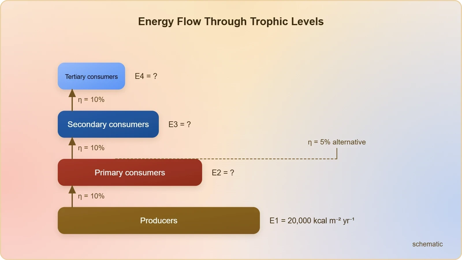
The calculation can be expressed compactly. If ##E_n## is the energy at trophic level ##n## and ##\eta## is the ecological efficiency, then:
This relationship shows that energy declines geometrically with trophic position. It also explains why food chains rarely exceed four or five levels: beyond that point, the energy available is too small to support a viable population. The same logic applies to the detritus chain, though its efficiency can differ because decomposers process material that has already been partially broken down.
Trophic Cascades and the Control of Ecosystem Structure
The flow of energy through trophic levels is not merely a passive accounting exercise; it actively shapes community structure. When a predator is removed or added, the effects can ripple through the food web in a phenomenon known as a trophic cascade. The classic example is the sea otter, sea urchin and kelp system of the North Pacific. Where otters are abundant, they control urchin numbers, allowing kelp forests to flourish. Where otters were hunted to near extinction, urchin populations exploded and kelp beds were reduced to barren grounds.

Top-Down and Bottom-Up Control
Ecologists distinguish two broad modes of control. Bottom-up control holds that the abundance of each trophic level is determined by the availability of resources from below, so adding nutrients increases producer biomass, which in turn supports more herbivores and carnivores. Top-down control holds that predators regulate the levels beneath them, so removing a top predator releases herbivores from limitation and can decimate producers. Most real ecosystems exhibit a blend of both, with the balance shifting seasonally and spatially.
The distinction has practical consequences for management. If a system is predominantly bottom-up, fertilisation or nutrient reduction will be the most effective lever. If it is top-down, predator conservation or reintroduction may be more powerful. The reintroduction of wolves to Yellowstone National Park is often cited as a top-down intervention, though the full story is more nuanced than popular accounts suggest, with climate, fire and other factors also playing roles.
Applying Cascade Theory to Real Food Webs
In the kelp forest, the cascade runs from otter to urchin to kelp, with consequences for fish, invertebrates and the broader community that depends on kelp structure. In the savanna, the relationship between lions, herbivores and grasses is complicated by migration, drought and fire, so simple cascade predictions must be tempered. In freshwater lakes, the addition of piscivorous fish can reduce zooplankton grazing on phytoplankton, sometimes improving water clarity, a principle used in lake restoration.
These examples show that energy flow and community structure are inseparable. The same trophic levels that organise energy transfer also organise the interactions that determine abundance. Recognising this unity is one of the most important conceptual advances in modern ecology, and it prepares learners for the next lesson, where the graphical representation of these relationships through ecological pyramids is examined in detail.
Common Misconceptions and Advanced Considerations
Several misconceptions recur in the study of energy flow. One is the belief that the ten per cent rule is a law of nature rather than a rough average. Another is the assumption that trophic levels correspond neatly to species, when in reality many organisms feed at multiple levels. A third is the confusion of biomass with energy, which leads to puzzlement over inverted biomass pyramids in aquatic systems. Addressing these misconceptions directly strengthens understanding and prepares learners for the more nuanced treatment of pyramids in the next lesson.
Why Inverted Biomass Pyramids Are Not Paradoxes
In the open ocean, the biomass of phytoplankton at any instant is often smaller than the biomass of the zooplankton that feed on them. This appears to violate the expectation that lower trophic levels hold more biomass, but the explanation lies in turnover rate. Phytoplankton reproduce and are consumed rapidly, so a small standing crop can support a much larger consumer biomass because the flow of energy through the producer level is high even though the stock is low. The pyramid of energy, which measures rates rather than stocks, remains upright.


This distinction between stock and flow is one of the most important quantitative insights in ecosystem ecology. It also explains why measuring biomass alone can mislead. A forest with a huge standing crop may have low annual productivity, while a pond with a tiny standing crop may be highly productive. Understanding the difference is essential for interpreting ecological pyramids correctly and for managing systems such as fisheries where turnover rates determine sustainable yields.
Humans as Omnivores Across Multiple Trophic Levels
Human beings illustrate the flexibility of trophic position. A diet rich in rice, wheat and vegetables places a person primarily at the second trophic level. Adding chicken or fish raises the effective position to the third, and eating predatory fish such as tuna pushes it higher still. Because humans are omnivores, they function at several trophic levels simultaneously, and the average trophic position of a population depends on its diet composition. This has implications for the energy cost of different food systems.
Diets based on plants require far less land and energy per calorie than diets based on top predators, precisely because of the losses at each transfer. This is the ecological logic behind arguments for reducing meat consumption, though the full picture involves cultural, economic and nutritional factors. For learners, the key point is that trophic position is a measurable property of diets and can be used to compare the efficiency of food systems across regions and income levels.
To consolidate these ideas, consider how a simple computational model can simulate energy flow. The following Python snippet calculates the energy available at each trophic level for a given efficiency and number of levels, illustrating the geometric decline described earlier.
def energy_flow(producer_energy, efficiency, levels):
    energies = [producer_energy]
    for _ in range(levels - 1):
        energies.append(energies[-1] * efficiency)
    return energies

for eta in (0.05, 0.10, 0.20):
    values = energy_flow(20000, eta, 4)
    print(f"Efficiency {eta:.0%}: {[round(v, 1) for v in values]}")
Running this code reproduces the figures in the worked example and allows learners to explore how sensitive top-level energy is to small changes in efficiency. Such models are deliberately simple, but they capture the essential arithmetic that underlies more elaborate ecosystem simulations. The next lesson will take these outputs and represent them as ecological pyramids, examining the three types and the conditions under which each can be inverted.
Synthesis and Key Takeaways
Energy flow through ecosystems is governed by two thermodynamic principles that together explain both the direction and the limits of biological activity. The first law guarantees that energy is conserved through its transformations, while the second law ensures that each transformation degrades some energy to heat. The result is a unidirectional flow from the sun, or from chemical gradients in hydrothermal vents, through producers to consumers, with a geometric decline at each step. This decline, quantified by ecological efficiency, sets the length of food chains and the abundance of top predators.
Trophic levels provide a functional framework for organising this flow, but they must be applied with awareness that organisms can occupy several levels at once. Grazing and detritus food chains represent two major pathways, with the former dominating in aquatic systems and the latter in terrestrial ones. Their interconnection produces food webs, which in turn support trophic cascades that shape community structure through both top-down and bottom-up control. These concepts are not merely descriptive; they inform conservation, fisheries management and agriculture.
Looking ahead, the next lesson will translate these energy relationships into ecological pyramids, examining the three types and the conditions under which each can be inverted. The quantitative skills developed here, particularly the ability to calculate energy at successive levels and to distinguish stock from flow, will be directly applied. Learners who master this lesson will be well prepared to evaluate the strengths and limitations of pyramid representations and to interpret real ecosystem data with confidence.
Also Read
- No links available.
From our network :
- Do You Need a New Router or Is Your Internet Plan the Problem?A practical comparison of the signs that point to router limits versus signs your broadband speed or provider is the bottleneck, so you can decide what to replace before spending money.
- AI-Powered 'Precision Diagnostic' Replaces Standard GRE Score ReportsDiscover the new GRE Precision Diagnostic. Learn how AI-powered behavioral analytics and time-to-solve tracking are replacing standard GRE score reports to empower students.
- Where to Put Your Wireless Router for Better CoverageA practical, physics-grounded guide to router placement: why the centre of the home beats the corner, how walls and metal sap signal, and how to run a simple survey that proves the improvement.
- Trump Political Strategy How Geopolitical Stunts Serve As Media Diversions
- How to Print Cheaply: Cutting the Cost per PageA practical, measured guide to lowering what each printed page costs — duplex and draft modes, third-party ink, yield mathematics, and knowing when a new printer beats refills.
- EV 2.0: The Solid-State Battery Breakthrough and Global Factory ExpansionDiscover the impact of the Solid-State Battery Breakthrough on the EV market. Learn about CATL and BYD stock growth, global factory expansion in Europe, and the future of EV 2.0 technology.
- Analyzing Trump Deportation Numbers Insights Into The 2026 Immigration Crackdown
- 98% of Global MBA Programs Now Prefer GRE Over GMAT Focus EditionExplore why 98% of global MBA programs now prefer the GRE over GMAT Focus. Learn about the shorter GRE format, verbal logic importance, and strategic versatility for students.
- 10 Physics Numerical Problems with Solutions for IIT JEEPrepare for IIT JEE with 10 physics numerical problems, complete with detailed solutions and conceptual explanations. Ideal for mastering kinematics, thermodynamics, electromagnetism, and optics.
RESOURCES
- Resources will be updated soon.