Trigonometry Meets Limits: Understanding the Sine Limit Formula

The Fundamental Sine Limit Formula

Defining the Core Ratio

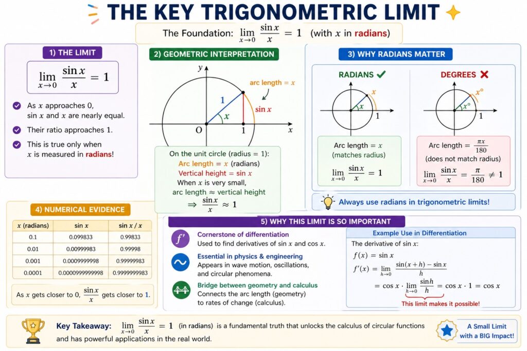
Trigonometric limits connect geometry and calculus. The most important formula involves the ratio of a sine function to its input variable. This relationship appears frequently in physics and engineering. We focus on the behavior of the ratio as the input approaches zero.

We analyze the behavior of ##\dfrac{\sin(x)}{x}## as ##x## approaches zero. This specific value serves as a foundation for many derivatives. Understanding this ratio is essential for advanced calculus courses. It represents the starting point for differentiating circular functions in mathematics.

The variable x must be measured in radians. Using degrees will change the limit value and break the standard formula. Always convert angles before performing any limit calculations in this context. Radians ensure the arc length matches the radius in the unit circle.

When x is very small, sin(x) and x are nearly equal. This proximity means their ratio stays close to one. We express this mathematically using the standard limit notation. This approximation is highly useful for simplifying complex equations in physical science.

This formula is the cornerstone of trigonometric differentiation. It allows mathematicians to find the rate of change for circular functions. Without it, the calculus of waves would be impossible. It bridges the gap between linear algebra and periodic motion.

The Problem of Indeterminate Forms

Direct substitution fails when we evaluate this limit at zero. If we plug in 0, we get sin(0) divided by 0. This results in the undefined expression 0/0. Calculus requires a more sophisticated approach to solve this specific problem.

Mathematicians call this result an indeterminate form. It suggests that a limit might exist, but algebra alone cannot find it. We need specific theorems to resolve this mystery. Indeterminate forms are common in calculus and require careful logical handling.

Simple division by zero is never allowed in mathematics. However, limits describe the behavior as we get closer to a point. They do not require us to reach the point itself. This distinction allows us to study functions where they are undefined.

We observe that as x shrinks, the gap between the numerator and denominator closes. Numerical tables show the value getting closer to one. This pattern suggests a clear horizontal asymptote. Visualizing this behavior helps students grasp the concept of convergence.

We must use geometric reasoning to prove the value is exactly one. This proof moves beyond simple arithmetic and looks at shapes. It provides a rigorous logical basis for the formula. Geometry offers the visual evidence that pure numbers sometimes hide.

Geometric Interpretation via the Unit Circle

Sector Areas and Triangles

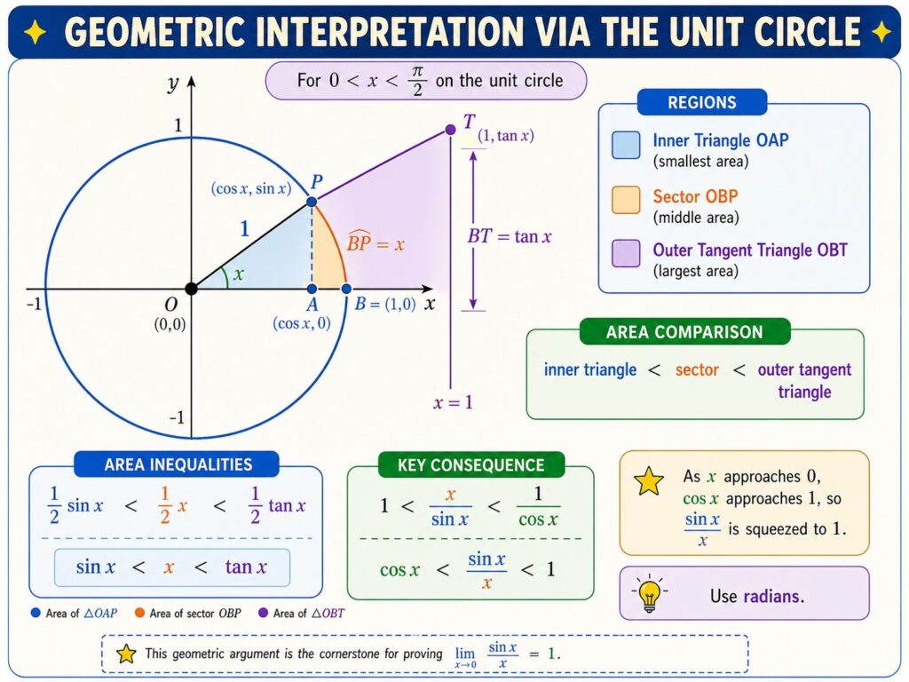
The unit circle provides a visual way to understand trigonometric limits. We draw a circle with a radius of 1 on a coordinate plane. This circle represents all possible sine and cosine values. It serves as our primary laboratory for geometric proofs.

Consider an angle ##x## in the first quadrant of the circle. This angle creates a triangle, a circular sector, and a larger external triangle. These three shapes have different but related areas. We use these areas to establish a mathematical hierarchy.

The height of the inner triangle represents ##\sin x##. The length of the circular arc is exactly ##x## units. Finally, the height of the outer tangent triangle is ##\tan x##. These lengths are the building blocks of our inequality chain.

We can compare the areas of these three geometric shapes. The inner triangle is the smallest, followed by the sector. The outer triangle is the largest of the three figures. This relationship remains true for all small positive values of ##x##.

This comparison creates a chain of inequalities. Since the areas depend on ##x##, we can relate the functions directly. This visual hierarchy is the first step in our proof. It allows us to bound the ratio between known functions.

Applying the Squeeze Theorem

The Squeeze Theorem helps us find limits by trapping a function. We place our target function between two other functions. If the outer functions meet, the inner one must follow. It is a powerful tool for solving difficult limits.

From our unit circle areas, we derive a specific inequality. We find that ##\cos x## is less than the ratio, which is less than ##1##. This holds true for small positive angles. The geometry dictates these strict mathematical boundaries.

As ##x## approaches zero, the value of ##\cos x## approaches one. The upper bound is already constant at one. Therefore, the function in the middle has nowhere else to go. Both sides "squeeze" the middle term toward a single value.

This logical "squeeze" forces the middle ratio to equal one. It is a powerful method for proving limits without using complex algebra. The geometry provides the necessary boundaries. It ensures that our limit is not just an estimate.

This proof is standard in introductory calculus textbooks. It demonstrates how geometry and limits work together. It confirms our numerical observations with absolute mathematical certainty. Mastery of this proof is a milestone for every calculus student.

Expanding Limits to Other Functions

Evaluating the Cosine Limit

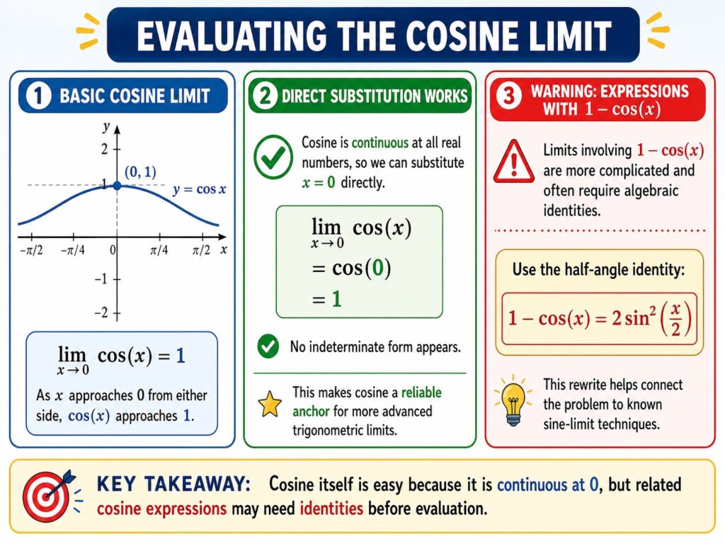
Other trigonometric functions have their own limit properties. For example, we often look at the limit of ##\cos x## as ##x## goes to zero. This limit is much simpler to evaluate than the sine limit. It follows standard continuity rules.

Direct substitution works for the cosine function because it is continuous. Since ##\cos(0)## equals ##1##, the limit is simply one. No indeterminate form appears in this basic case. This simplicity makes it a reliable anchor for more complex problems.

However, limits involving ##1 - \cos x## are more complex. These often appear in physics problems involving pendulums or springs. They require different algebraic identities to solve properly. We must transform them into forms we can easily calculate.

We often use the half-angle identity to rewrite cosine terms. This transformation allows us to use the sine limit formula we already know. It bridges the gap between different functions. Substitution remains a key strategy for handling these variations.

Understanding the behavior of cosine helps in analyzing wave phases. It ensures that we can handle any trigonometric expression in a limit. Consistency across functions is key for calculus. It allows for a unified theory of trigonometric behavior.

Transforming Tangent Limits

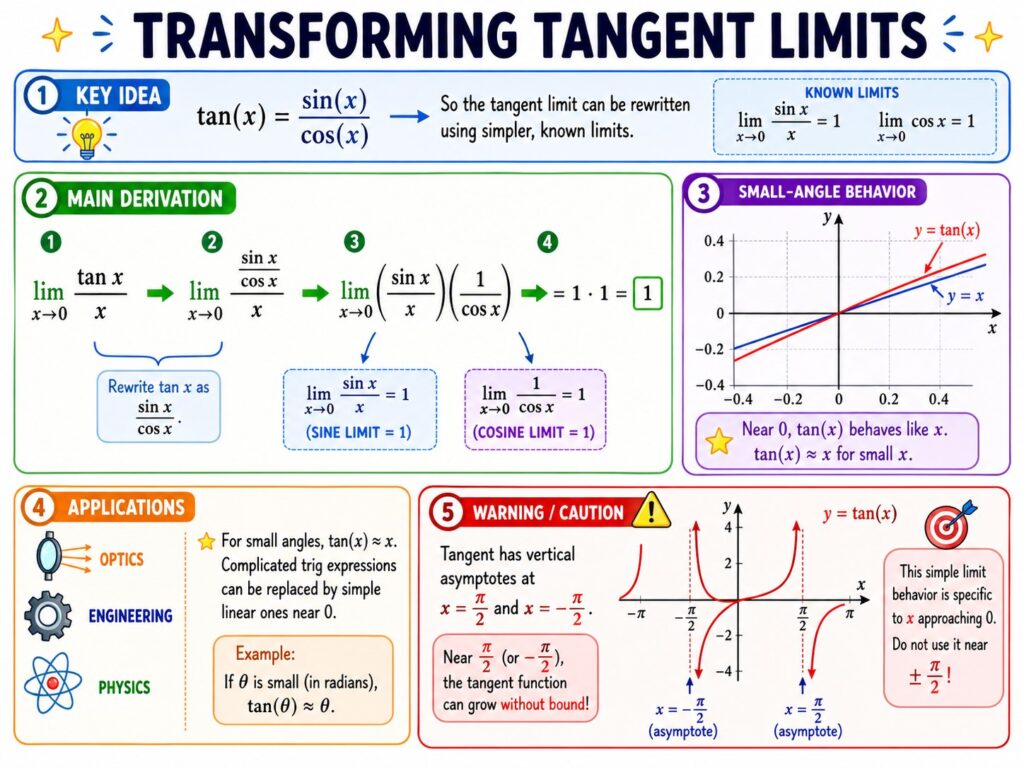
The tangent function also has a predictable limit at zero. We define tan(x) as the ratio of sin(x) to cos(x). This definition helps us evaluate its limit. We break the complex function into its simpler components.

When we divide tan(x) by x, we can split the fraction. We get the sine limit multiplied by the reciprocal of cosine. Both parts are easy to manage. This decomposition is a standard technique in limit evaluation.

Since the sine limit is one and the cosine limit is one, the result is one. This means tan(x) and x behave similarly near zero. They are essentially interchangeable for small values. This observation simplifies many engineering calculations.

This property is useful in optics and small-angle approximations. Scientists replace complex trigonometric functions with simple linear variables. This simplification makes hard equations much easier to solve. It reduces computational load without losing significant accuracy.

We must be careful when x approaches other values like ##\dfrac{\pi}{2}##. Tangent has vertical asymptotes where the limit might be infinite. Always check the target value before calculating. Understanding the domain is as important as the limit itself.

Practical Problem Solving and Applications

Algebraic Manipulation Techniques

Solving limit problems often requires changing the variable's coefficient. For example, we might see sin(4x) divided by x. This requires a technique called balancing the denominator. We must make the arguments of the function match.

We multiply the top and bottom by the same constant. This ensures that the argument inside the sine matches the denominator. Once they match, we can apply our standard formula. It is a simple but effective algebraic trick.

Substitution is another helpful tool for solving complex limits. We can replace a group of terms with a single variable ##u##. This simplifies the appearance of the limit expression. It helps us see the underlying structure of the problem.

Always remember that if ##x## goes to zero, then ##4x## also goes to zero. This allows us to maintain the validity of the limit. It is a standard trick in calculus exams. Consistency in the approach leads to fewer errors.

Computational Verification

Trigonometric limits are not just theoretical exercises. They describe how physical systems behave when changes are very small. This is vital in fields like structural engineering. Limits help predict how materials respond to tiny stresses.

In electronics, these limits help define the behavior of alternating currents. Signal processing relies on the smooth transitions of sine and cosine waves. Limits ensure these models remain continuous. They prevent mathematical gaps in our physical descriptions.

Computer graphics use these formulas to render smooth curves. When zooming into a circle, the segments look like straight lines. This is a direct application of the sine limit. It allows computers to simulate realistic shapes efficiently.

We can verify these limits using simple computer programs. Coding allows us to test values closer to zero than a calculator can handle. It provides an experimental view of math. This bridge between theory and code strengthens understanding.

import math

def check_limit(x_val):
    # Calculate the ratio of sin(x) to x
    return math.sin(x_val) / x_val

for i in range(1, 6):
    small_x = 10**(-i)
    print(f"x: {small_x}, ratio: {check_limit(small_x)}")

This intersection of trigonometry and limits is a gateway to higher math. It prepares students for derivatives, integrals, and series. Every step builds on these fundamental ratios. Mastery of these concepts ensures success in all future calculus topics.