The Algebra of Limits: Rules and Applications

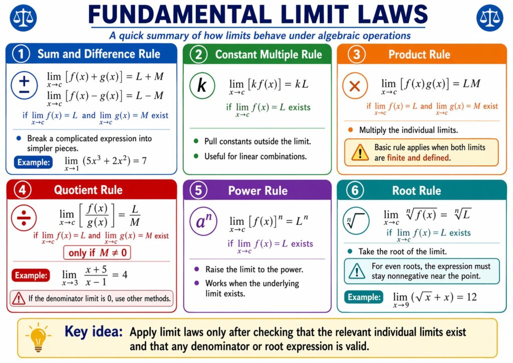
Fundamental Limit Laws for Sums and Differences

Addition Rules in Calculus

The addition rule simplifies the process of finding the limit of two functions added together. It states that the limit of a sum is equal to the sum of the individual limits. This rule applies when both limits exist.

We use this property to break down polynomial expressions into smaller components. If we have ##f(x)## and ##g(x)##, we calculate their limits at a specific point ##c## separately. This modular approach reduces the chance of making calculation errors.

Mathematically, the rule is expressed using standard limit notation. If ##\lim_{x \to c} f(x) = L## and ##\lim_{x \to c} g(x) = M##, then the sum is simply ##L + M##. This linear property is a cornerstone of basic calculus.

Consider a practical example where two different physical forces act on a single point. You find the limit of each force as the point approaches a boundary. Adding these limits gives the total limit of the combined force system.

Students must confirm that each function is well-behaved near the point of interest. If either limit results in an undefined value, the addition rule cannot be applied directly. Always verify the existence of individual limits before performing the addition.

Subtraction Rules and Constant Multiples

The subtraction rule works identically to the addition rule but involves finding the difference between two limits. It allows mathematicians to evaluate the limit of ##f(x) - g(x)## by subtracting the limit of ##g(x)## from ##f(x)##.

This rule is essential for finding the rate of change or the difference between two converging sequences. Like the addition rule, it requires that both functions have finite limits at the target value ##c## to be valid.

Constant multiples are also handled through a similar algebraic property. If a function is multiplied by a constant ##k##, the limit of the product is ##k## times the limit of the function. This scales the limit value.

Combining subtraction and constant multiples allows for the evaluation of complex linear combinations. You can pull constants outside the limit operator to simplify the expression. This makes the remaining algebraic work much easier to manage and solve.

Always maintain the order of operations when applying the subtraction rule. Reversing the order of functions will change the sign of the final limit result. Accuracy in sign placement prevents common mistakes in multi-step calculus homework problems.

Rules for Multiplication and Division

Product Rule for Limits

The product rule for limits states that the limit of a product is the product of the individual limits. This applies when you multiply two functions, ##f(x)## and ##g(x)##, as ##x## approaches a specific value ##c##.

If the individual limits exist and are finite, you simply multiply the two resulting numbers. This property is particularly useful when dealing with terms like ##x \cdot \sin(x)## or other products of basic functions in algebraic expressions.

Calculus students use this rule to handle higher-degree polynomials by treating them as products of linear factors. It simplifies the evaluation process by focusing on one factor at a time. This step-by-step method ensures clarity during derivation.

In physics, the product rule helps determine the limit of quantities like work, which is force times displacement. If both force and displacement approach specific limits, their product defines the limit of the work done by the system.

Be careful when one of the limits is zero and the other is infinite. This creates an indeterminate form that requires more advanced techniques like L'Hôpital's Rule. The basic product rule only works for finite, well-defined limit values.

Quotient Rule and Constraints

The quotient rule allows for the calculation of the limit of a fraction. The limit of a quotient is the quotient of the limits, provided the limit of the denominator is not equal to zero at that point.

To apply this rule, you evaluate the limit of the numerator and the denominator separately. If the denominator’s limit is non-zero, you divide the top result by the bottom result to find the final answer for the expression.

When the denominator approaches zero, the quotient rule cannot be used directly. This situation often indicates a vertical asymptote or a hole in the graph. You must perform algebraic simplification, such as factoring, to resolve these cases.

Rationalization is another technique used when the quotient rule fails due to a zero denominator. By multiplying by the conjugate, you can often cancel out the problematic terms. This reveals the true limit hidden within the initial fraction.

The quotient rule is vital in economics for calculating marginal costs and average rates. It helps analysts understand how ratios behave as variables approach specific thresholds. Mastery of this rule is necessary for any advanced mathematical study.

Power and Root Rules for Limits

Power Rule Applications

The power rule for limits is used when a function is raised to a constant exponent ##n##. It states that the limit of a function raised to a power is the limit itself raised to that power.

This rule applies to both positive and negative integer exponents. If ##\lim_{x \to c} f(x) = L##, then ##\lim_{x \to c} [f(x)]^n = L^n##. This significantly speeds up the calculation of limits involving squared or cubed terms.

Engineers use the power rule when calculating areas and volumes that depend on a variable approaching a limit. For example, if the radius of a circle approaches a value, the power rule helps find the limit of the area.

You must ensure that the base function has a defined limit before applying the exponent. If the base limit is negative and the exponent is a fraction, the result might involve complex numbers. This requires careful domain checking.

The rule also extends to cases where the exponent is a real number. As long as the expression is defined within the real number system, the power rule remains a reliable tool for simplifying various types of calculus problems.

Root Rule and Domain Restrictions

The root rule is a specific case of the power rule where the exponent is a fraction. It states that the limit of a root of a function is the root of the limit of that function.

When applying the root rule, you must consider the index of the root. For even roots, like square roots, the limit of the inner function must be non-negative. Negative values under even roots are not defined for real limits.

If the index of the root is odd, like a cube root, the limit can be any real number. Odd roots are defined for both positive and negative values. This distinction is critical when solving limits involving radical expressions.

Using the root rule helps simplify complex limits involving nested radicals. By moving the limit operator inside the root sign, you can solve the inner algebraic expression first. This hierarchical approach clarifies the path to the final solution.

Always verify the domain of the function near the limit point. If the function is undefined on one side of the point, you might need to check one-sided limits. The root rule remains valid within the function's natural domain.

Practical Examples and Problem Solving

Step-by-Step Limit Evaluation

Successful limit evaluation requires a systematic application of the rules discussed. Start by identifying the structure of the function, such as whether it is a sum, product, or quotient. This determines which algebraic rule to apply first.

Substitute the value of ##x## directly into the expression to see if it yields a defined number. If direct substitution works, the function is continuous at that point. The algebraic rules confirm why this simple substitution is mathematically sound.

If direct substitution leads to a defined value, you have found the limit. Most basic polynomial and rational functions behave predictably. The algebra of limits provides the formal proof for these intuitive results in standard calculus exercises.

When facing multi-part functions, apply the addition and subtraction rules to separate the terms. Then, use the constant multiple and power rules on each individual term. This granular analysis prevents errors in complex algebraic manipulations.

Practice with various functions to build intuition for which rule to use. Over time, you will recognize patterns in rational and radical functions. This recognition allows you to solve limits more quickly during timed exams or professional tasks.

Common Pitfalls and Indeterminate Forms

One common mistake is applying the quotient rule when the denominator limit is zero. This leads to an undefined expression rather than a numerical limit. Always check the denominator before finalizing your division in limit problems.

Indeterminate forms like ##\dfrac{0}{0}## or ##\dfrac{\infty}{\infty}## require algebraic manipulation before applying the rules. You might need to factor the numerator and denominator to cancel out common terms. This step is necessary to remove the source of the indeterminacy.

Another pitfall is forgetting the domain restrictions of the root rule. Applying a square root rule to a negative limit will result in an error in the real number system. Always validate the sign of the inner limit first.

Ensure that the limit exists from both the left and the right sides. If the one-sided limits are different, the overall limit does not exist. The algebraic rules assume that a single, consistent limit value exists at the point.

Finally, keep your work organized when dealing with nested functions. Apply the outermost rule first and work your way inward. This structured method ensures that every part of the algebra of limits is applied correctly to the problem.