On This Page
The Intuitive Meaning of Approach
Visualizing Proximity
A limit describes the behavior of a function as the input ##x## approaches a specific value ##a##. We do not care about the value exactly at ##a##. Instead, we observe the trend of the output values ##f(x)##.
Imagine walking along a path toward a specific destination. Your position represents the output of the function. Even if the destination is a hole in the ground, you can still describe where you were headed before you arrived.
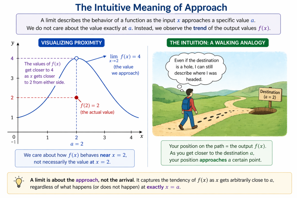
The walking path analogy helps visualize the idea of approach in an intuitive way.
In mathematics, this "heading" is the limit. We use the notation
to express this idea. It states that as ##x## gets closer to ##a##, the function value ##f(x)## gets closer to ##L##.
Proximity is key to understanding this concept. We look at values like ##a + 0.1##, ##a + 0.01##, and ##a + 0.001##. By testing these numbers, we see if the function settles on a single, predictable value from both sides.
This process allows mathematicians to handle functions that are undefined at certain points. It provides a way to talk about continuity and change. Without limits, the entire field of calculus would lack a rigorous logical foundation for its operations.
Left-Hand and Right-Hand Limits
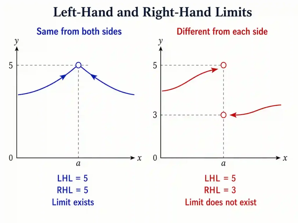
To say a limit exists, the function must approach the same value from both directions. The left-hand limit tracks the function as ##x## moves from smaller values toward ##a##. We write this as
The right-hand limit tracks the function as ##x## moves from larger values toward ##a##. We write this as
Both directions must agree for the general limit to be considered valid and defined.
If the left-hand limit is ##5## and the right-hand limit is ##5##, then the overall limit is ##5##. If they differ, the limit does not exist at that specific point. This often happens at jumps or breaks in a graph.
Think of two people walking toward each other on a bridge. If they meet at the same point, the limit is that meeting spot. If one person is on a higher level than the other, they never meet.
In technical terms, we say the limit exists if and only if the left-hand and right-hand limits are equal. This requirement ensures that the function's behavior is consistent. It is a fundamental rule for analyzing function continuity.
Distinguishing f(a) from the Limit
The Concept of a Hole in the Graph
The value ##f(a)## is what the function actually equals at ##x = a##. The limit is what the function "intends" to be. Sometimes these two values are the same, but in many interesting calculus problems, they are different.
A "hole" occurs when a function is undefined at a specific point but behaves smoothly everywhere else. For example, a rational function might have a factor that cancels out. This leaves a gap in the line at that coordinate.
Even if ##f(a)## does not exist, the limit can still exist. The limit tells us the height of the hole. It describes the surrounding neighborhood of the point. We use algebra to "fill" the hole and find the value.
Consider a function where you cannot plug in ##x = 2## because it causes division by zero. By looking at values very close to ##2##, we find the trend. The limit gives us the answer that direct evaluation cannot.
This distinction is the heart of calculus. Limits allow us to work with "almost zero" or "almost infinity." We bypass the restrictions of basic arithmetic to see the bigger picture of how a curve flows through space.
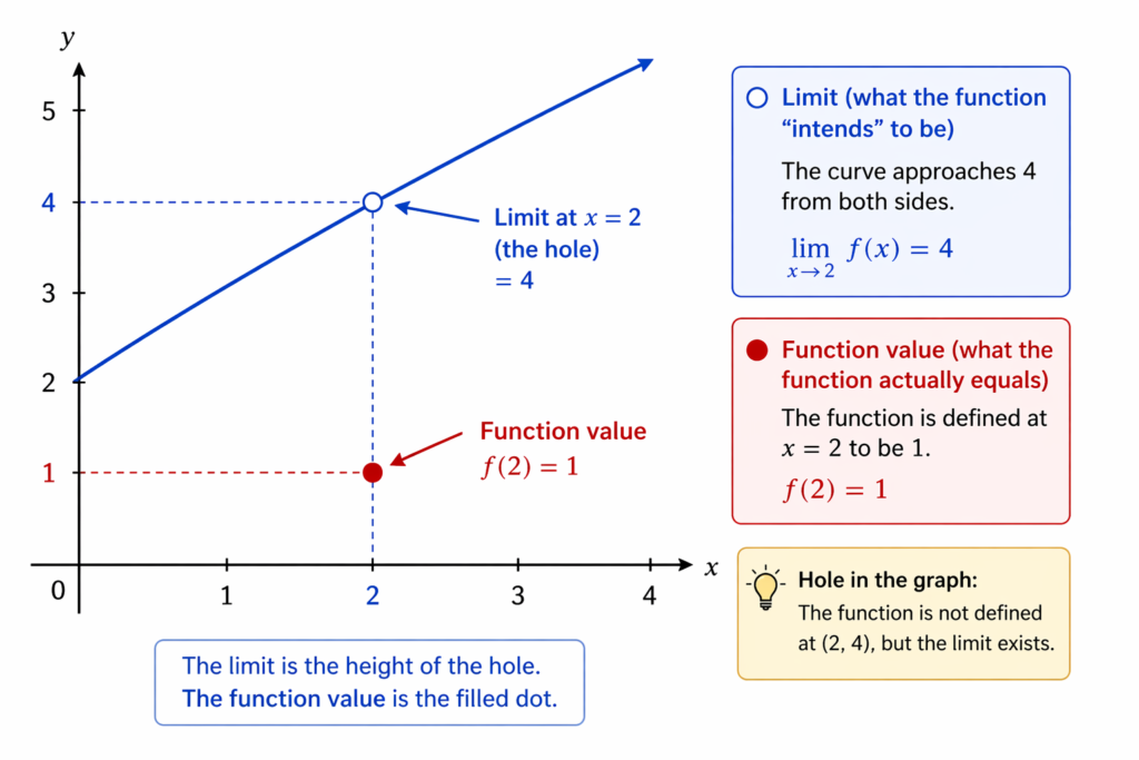
It shows that the limit exists at the hole even though the function value is different
Find the limit of the function as ##x## approaches ##2##:
Piecewise Functions and Discontinuity
Piecewise functions often show the difference between ##f(a)## and the limit. A function might be defined as ##y = 1## for all ##x## except at ##x = 0##, where it is defined as ##y = 5##.
In this case, the limit as ##x## approaches ##0## is ##1##. However, the actual function value ##f(0)## is ##5##. The graph has a single dot floating above a straight line. The limit ignores that specific dot.
This separation is called a removable discontinuity if the limit exists. If the limit does not exist, such as a jump between two different lines, it is a non-removable discontinuity. Limits help us categorize these different types of breaks.
Engineers use this to model systems that change state instantly. While the physical world rarely has true gaps, mathematical models use them to simplify complex shifts. Understanding the limit helps predict the system's state before the shift.
Always check both the limit and the function value when analyzing a point. If they are equal, the function is continuous at that point. If they differ, you have found a point of interest that requires further investigation.
Graphical Representation of Limits
Reading Limits from a Curve
To find a limit graphically, place your finger on the curve to the left of ##x = a##. Slide your finger along the curve toward the vertical line ##x = a##. Note the height your finger is approaching.
Repeat this process from the right side of ##x = a##. If both fingers approach the same height ##L##, then ##L## is the limit. This visual method is the most intuitive way to understand the concept for beginners.
If there is a solid dot at a different height, ignore it. If there is an open circle at that height, the limit is still that height. The graph shows the "path" the function takes toward the target value.
A graph can also show if a limit does not exist. If the curve oscillates wildly as it gets closer to a point, it never settles. If the two sides of the curve go to different heights, they disagree.
Visualizing limits helps build a mental map of function behavior. It turns abstract algebraic symbols into physical shapes. Most students find that seeing the "approach" on a coordinate plane makes the formal definitions much easier to grasp.
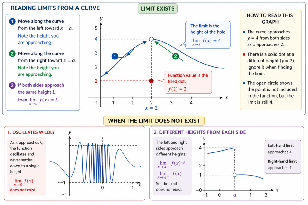
It also contrasts this with two common cases where a limit does not exist.
Identifying Vertical and Horizontal Asymptotes
Asymptotes represent limits involving infinity. A vertical asymptote occurs when the function values grow without bound as ##x## approaches a finite number. We say the limit is positive or negative infinity in these specific cases.
For example, the function ##\dfrac{1}{x^2}## shoots upward as ##x## gets closer to zero. The limit from both the left and the right is infinity. This tells us the graph has a vertical asymptote at the y-axis.
Horizontal asymptotes describe the limit as ##x## goes to infinity or negative infinity. This shows the "end behavior" of the function. It tells us what value the function settles on as the input becomes very large or small.
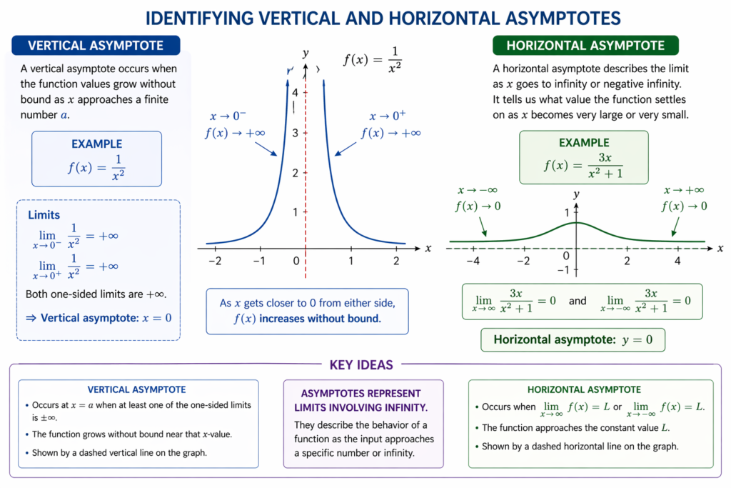
It helps distinguish vertical asymptotes from horizontal asymptotes visually.
Determine the limit of the following function as ##x## approaches zero:
Graphing these features allows us to understand the constraints of a function. We can see where the function is "blocked" or where it levels out. These visual cues are essential for sketching complex equations without calculating every point.
Limits at infinity are particularly useful in science. They help predict the long-term stability of a population or the final temperature of an object. The horizontal asymptote represents the equilibrium state of the mathematical model.
Mathematical Formalization and Indeterminate Forms
The Delta-Epsilon Concept Simplified
While intuition is helpful, mathematicians need a strict definition. This is provided by the ##\epsilon-\delta## (epsilon-delta) proof. It defines the limit based on the distance between the function and the limit value ##L##.
For every small distance ##\epsilon## we choose around the limit ##L##, there must be a corresponding distance ##\delta## around the point ##a##. This ensures that all function values within ##\delta## fall within the ##\epsilon## range.
In simpler terms, if you want to be "this close" to the limit, you must stay "this close" to the target ##x## value. This rigorous definition removes ambiguity. It proves that the approach is consistent and mathematically sound.
Most introductory courses focus on the intuition, but the formal definition is what makes calculus work. It allows us to prove theorems about derivatives and integrals. It is the language of precision in modern mathematical analysis.
Understanding this concept helps you realize that limits are not just guesses. They are precisely defined boundaries. Even if we cannot reach a value, we can define exactly how close we can get to it.
Handling the 0/0 Scenario
When plugging ##a## into a function results in ##\dfrac{0}{0}##, we call it an indeterminate form. This does not mean the limit does not exist. It means the current form of the expression is hiding the answer.
Algebraic techniques like factoring, rationalization, and simplification are used to reveal the limit. By removing the common factor that causes the zero, we can see the true behavior of the function at that point.
These scenarios often appear in physics when calculating instantaneous velocity. We are looking at a change in position over a change in time as time approaches zero. Limits provide the only way to solve this.
Mastering these techniques is essential for progressing in calculus. It requires a strong foundation in algebra and a clear understanding of the limit concept. Each indeterminate form is a puzzle that reveals a hidden value.
Evaluate the limit using rationalization:
Through these methods, we find that ##\dfrac{0}{0}## can represent any real number. The limit process extracts the specific value relevant to the function. It is a powerful tool for analyzing rates of change and steepness.
RESOURCES
- ELI5: What is a limit in calculus? : r/explainlikeimfive - Reddit
- What exactly are the ship Class and Block limits?
- What exactly are the limits of the Chaos Gods? : r/40kLore - Reddit
- What exactly is the limit on Wyvern Levels? - ARK News
- What exactly is the limit to the Public Domain? - Reddit
- The moral limits of what, exactly? | Economics & Philosophy
- What exactly is the limit on "pro" and how much more is it than free?
- Limits intro (article) - Khan Academy
- What exactly is the Meta AI generation limit? - 1354241
- What exactly is "No limit Fallacy" ? Can Anyone help me, Please?
- What exactly is going on when we're finding a limit?
- What exactly are the limits to paying out workers on Roblox?
- What exactly is the speed limit on roads where no speed ... - Facebook
- What exactly MAX_UNIFORM_BLOCK_SIZE limits? - Google Groups
- What exactly do --limit 1/s and --limit-burst mean in iptables rules?
0 Comments