
On This Page
- Introduction to Asymptotes
- Understanding Vertical Asymptotes
- Calculating Vertical Asymptotes
- Logarithmic Functions And Vertical Asymptotes
- Visual Illustration Of A Vertical Asymptote
- Additional Practice Problems
- Points To Remember
- Understanding Horizontal Asymptotes
- Calculating Horizontal Asymptotes
- Graphing Rational Functions With Asymptotes
- Programming Solutions For Asymptotes
- Real-World Applications And Advanced Concepts
- Additional Practice Problems
- Points To Remember
Introduction to Asymptotes
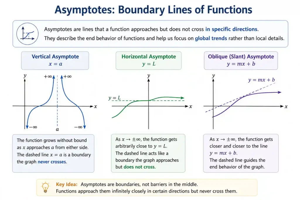
Asymptotes serve as boundary lines that functions approach but rarely cross in specific directions. They define the long-term behavior of mathematical models, especially when dealing with rational expressions. Understanding these boundaries is essential for sketching curves and predicting system stability.
In professional mathematical analysis, identifying these lines allows researchers to simplify complex functions. By focusing on asymptotic behavior, we can ignore local fluctuations and concentrate on the global trends. This perspective is vital in fields ranging from physics to financial forecasting.
They help describe how a graph behaves near critical values or far away from the origin.
This figure explains asymptotes as boundary lines that functions approach in specific directions. It shows vertical, horizontal, and oblique asymptotes with separate coordinate-plane examples. The diagrams help students understand how asymptotes describe long-term graph behavior and simplify the study of complex functions.
Defining Asymptotic Behavior
Asymptotic behavior refers to the trend of a function as the input variables approach specific values or infinity. It describes how a curve stabilizes or explodes at the boundaries of its domain. This behavior is formally analyzed using limit notation in calculus.
Engineers use these definitions to determine the limits of physical systems, such as electrical circuits or structural loads. By defining how a system behaves at its extremes, we can prevent failures and optimize performance. It is the cornerstone of stability analysis.
Graphical Representation
Visually, an asymptote appears as a straight line that the graph of a function gets closer to as it moves. While the curve may look like it touches the line, it typically stays infinitely close without intersection. This visualization aids in conceptualizing infinite growth.
In digital plotting, representing these lines correctly is crucial for clear communication. Professional graphs often use dashed lines to distinguish asymptotes from the actual function curve. This clarity helps in identifying discontinuities and end-behavior trends at a quick glance.
Importance in Calculus
Calculus relies heavily on asymptotes to describe limits and continuity across the real number line. They provide a framework for understanding how functions behave near points of division by zero. This knowledge is required for solving advanced integration and differentiation problems.
Beyond pure mathematics, calculus-based asymptotes are used in machine learning to understand loss functions. As optimization algorithms converge, they often follow asymptotic paths toward a minimum value. Mastering these concepts provides a deeper insight into algorithm convergence and efficiency.
Understanding Vertical Asymptotes
Vertical asymptotes occur at specific x-values where the function's output increases or decreases without bound. These lines represent points of essential discontinuity where the function is undefined. They are typically found in rational functions where the denominator equals zero.
Identifying these vertical lines is the first step in mapping the domain of a function. They indicate where a function "breaks," creating separate branches on the coordinate plane. Understanding these breaks is critical for ensuring that mathematical models remain valid within their intended scope.
Formal Definition
A vertical asymptote is formally defined using one-sided limits as the variable approaches a constant ##c##. If the function approaches infinity from either the left or the right, the line ##x = c## is an asymptote. This definition covers all possible infinite discontinuities.
Mathematically, this implies that the function grows infinitely large in magnitude as it nears the vertical line. This property is unique to vertical asymptotes and distinguishes them from holes in a graph. Holes occur when the limit exists but the function is undefined.
Identifying Discontinuities
To find vertical asymptotes in rational functions, one must look for values that make the denominator zero. However, it is essential to ensure these values do not also make the numerator zero. If both are zero, a hole might exist instead.
Professional analysis involves factoring both the numerator and the denominator to cancel common terms. Once the function is in its simplest form, the remaining zeros of the denominator indicate the locations of the vertical asymptotes. This systematic approach prevents errors in graphing.
Limits at Infinity
While vertical asymptotes are defined by limits resulting in infinity, they are distinct from horizontal asymptotes. They focus on what happens as the input approaches a finite value. This distinction is fundamental for students learning the nuances of limit theory.
In computational mathematics, handling these limits requires symbolic logic to avoid floating-point errors. Software like SymPy can evaluate these limits precisely, identifying the exact location of vertical boundaries. This precision is necessary for developing robust scientific software and simulation tools.
Calculating Vertical Asymptotes
Calculating vertical asymptotes requires algebraic manipulation and a solid grasp of function domains. For rational functions, the process is straightforward but requires attention to detail regarding simplification. For transcendental functions, the behavior is often periodic or logarithmic in nature.
The calculation process serves as a diagnostic tool for understanding function constraints. By identifying where a function fails, we can define the safe operating parameters for engineering models. This analytical rigor is a hallmark of professional mathematical practice and applied science.
Rational Functions
For a rational function ##R(x) = P(x)/Q(x)##, the vertical asymptotes are found by studying the denominator after the function has been simplified. A vertical asymptote appears at an ##x## value where the denominator becomes zero and the numerator does not cancel that same factor. Therefore, the first step is to simplify the rational expression, and the second step is to solve ##Q(x) = 0## for the remaining denominator.
These ##x## values are excluded from the domain of the function. Near such a point, the graph usually rises or falls without bound. This behavior is written using one-sided limits, because the function may approach positive infinity from one side and negative infinity from the other side.
###\lim_{x \to c^+} f(x) = \pm\infty \quad \text{or} \quad \lim_{x \to c^-} f(x) = \pm\infty###
Vertical Asymptotes Of Rational Functions
Consider the function ##f(x) = \frac{5}{x-3}##. The denominator is ##x - 3##. To find the excluded value, set the denominator equal to zero:
###x - 3 = 0 \implies x = 3###
Since the numerator ##5## is a nonzero constant, the factor ##x - 3## does not cancel. Therefore, ##x = 3## is a vertical asymptote. As ##x## approaches ##3## from the right, the denominator is a small positive number, so the function becomes very large and positive. As ##x## approaches ##3## from the left, the denominator is a small negative number, so the function becomes very large and negative.
###\lim_{x \to 3^+} \frac{5}{x-3} = +\infty \quad \text{and} \quad \lim_{x \to 3^-} \frac{5}{x-3} = -\infty###
| Step | Mathematical Action | Meaning |
|---|---|---|
| 1. Identify denominator | For ##R(x)=P(x)/Q(x)##, study ##Q(x)## | The denominator controls where the function may become undefined. |
| 2. Simplify first | Cancel common factors, if any | Cancelled factors usually create holes, not vertical asymptotes. |
| 3. Solve denominator | Set ##Q(x)=0## | The solutions give excluded ##x## values. |
| 4. Check remaining factors | See whether the zero still remains in the denominator | If the factor remains, the value is a vertical asymptote. |
Example: Solving A Denominator Equation
Suppose the denominator of a rational function contains the expression ##x^2 - 4##. To find possible vertical asymptotes, solve the equation ##x^2 - 4 = 0##. This expression is a difference of squares, so it factors neatly.
The values ##x = 2## and ##x = -2## are possible vertical asymptotes. They become actual vertical asymptotes only if the factors ##(x-2)## and ##(x+2)## remain in the denominator after simplification.
Logarithmic Functions And Vertical Asymptotes
Logarithmic functions also have vertical asymptotes, but the reason is slightly different. For ##f(x) = \ln(x)##, the input ##x## must be positive. The logarithm is undefined at ##x = 0## and for negative ##x## values. As ##x## approaches ##0## from the right, the value of ##\ln(x)## decreases without bound.
Therefore, the graph of ##f(x) = \ln(x)## has a vertical asymptote at ##x = 0##. Unlike many rational functions, we only approach this asymptote from the right because the natural logarithm is not defined for negative real inputs.
Shifted Logarithmic Functions
For transformed logarithmic functions such as ##f(x) = \log(x-h)##, the domain begins where the inside expression becomes positive. The boundary occurs when ##x-h=0##. Therefore, the vertical asymptote shifts from ##x = 0## to ##x = h##.
The boundary of the domain is ##x = -5##. Since ##\ln(x+5)## becomes undefined at that boundary and approaches negative infinity from the right side, the vertical asymptote is:
| Function Type | Domain Condition | Vertical Asymptote |
|---|---|---|
| Basic logarithm | For f(x) = ln(x), require x > 0 |
x = 0 |
| Right-shifted logarithm | For f(x) = ln(x - h), require x - h > 0 |
x = h |
| Left-shifted logarithm | For f(x) = ln(x + 5), require x + 5 > 0 |
x = -5 |
| General log expression | For f(x) = log(g(x)), require g(x) > 0 |
Boundary values where g(x) = 0 |
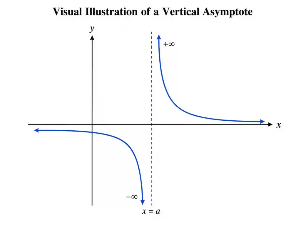
Visual Illustration Of A Vertical Asymptote
The following simple plot illustrates how the graph of ##f(x)=\frac{5}{x-3}## behaves near the vertical asymptote ##x=3##. The dashed vertical line represents the asymptote. The two branches of the curve move in opposite infinite directions as they approach this line.
Python Code For Generating The Plot
The following Python code can be used to generate a clearer mathematical plot of ##f(x)=\frac{5}{x-3}##. The code avoids drawing the function exactly at ##x=3## because the function is undefined there.
import numpy as np
import matplotlib.pyplot as plt

# Function definition
def f(x):
    return 5 / (x - 3)

# Create x-values on both sides of the vertical asymptote
x_left = np.linspace(-5, 2.9, 400)
x_right = np.linspace(3.1, 8, 400)

# Plot the two branches separately
plt.figure(figsize=(7, 4))
plt.plot(x_left, f(x_left), label="f(x) = 5/(x - 3)")
plt.plot(x_right, f(x_right))

# Draw the vertical asymptote
plt.axvline(x=3, linestyle="--", label="Vertical asymptote: x = 3")

# Improve readability
plt.ylim(-30, 30)
plt.axhline(y=0, linewidth=0.8)
plt.xlabel("x")
plt.ylabel("f(x)")
plt.title("Vertical Asymptote of f(x) = 5/(x - 3)")
plt.legend()
plt.grid(True)

plt.show()
Additional Practice Problems
Problem 1: Rational Function
Find the vertical asymptotes of the function:
First, factor the denominator:
Now set each factor equal to zero:
Since the numerator ##2x+1## does not cancel either denominator factor, both values are vertical asymptotes.
Problem 2: Hole Or Vertical Asymptote?
Determine whether ##x=2## is a hole or a vertical asymptote for the function:
The factor ##x-2## appears in both numerator and denominator, so it cancels:
Because the factor ##x-2## cancels, ##x=2## is not a vertical asymptote. It is a hole. The remaining denominator ##x+4## gives a vertical asymptote at ##x=-4##.
Problem 3: Logarithmic Function
Find the vertical asymptote of:
The input of the logarithm must be positive:
The boundary of the domain is ##x=7##. Therefore, the vertical asymptote is:
| Function | Critical Equation | Result |
|---|---|---|
5 / (x - 3) |
x - 3 = 0 |
Vertical asymptote at x = 3 |
(2x + 1) / (x² - 9) |
x² - 9 = 0 |
Vertical asymptotes at x = 3 and x = -3 |
(x - 2) / ((x - 2)(x + 4)) |
Cancel x - 2, then solve x + 4 = 0 |
Hole at x = 2, vertical asymptote at x = -4 |
ln(x - 7) |
x - 7 > 0 |
Vertical asymptote at x = 7 |
Points To Remember
- For rational functions, simplify first before identifying vertical asymptotes.
- Zeros of the remaining denominator usually produce vertical asymptotes.
- Cancelled denominator factors usually produce holes instead of asymptotes.
- For logarithmic functions, solve the inside expression boundary, usually where the logarithm input becomes zero.
- One-sided limits are important because the left-hand and right-hand behavior near a vertical asymptote may be different.
Trigonometric Functions
Trigonometric functions such as tangent, cotangent, secant, and cosecant have periodic vertical asymptotes. These asymptotes occur because the functions are defined using ratios involving sine and cosine. Whenever the denominator of such a ratio becomes zero, the function becomes undefined and may approach positive or negative infinity.
For ##\tan(x)##, the definition is based on the ratio ##\tan(x)=\frac{\sin(x)}{\cos(x)}##. Therefore, tangent is undefined wherever ##\cos(x)=0##. These points occur at odd multiples of ##\frac{\pi}{2}##, giving a repeating pattern of vertical asymptotes across the graph.
This means the graph of ##\tan(x)## has vertical asymptotes at ##x=\frac{\pi}{2}##, ##x=\frac{3\pi}{2}##, ##x=-\frac{\pi}{2}##, and so on. The integer ##n## represents the periodic repetition of these asymptotes in both directions along the ##x##-axis.
Analyzing these periodic boundaries is important in signal processing, wave mechanics, and electrical systems. In these fields, trigonometric functions often model oscillations. The vertical asymptotes mark values where a mathematical model may become unstable, undefined, or physically unrealistic.
| Function | Undefined When | Vertical Asymptotes |
|---|---|---|
tan(x) = sin(x) / cos(x) |
cos(x) = 0 |
x = π/2 + nπ, n ∈ Z |
sec(x) = 1 / cos(x) |
cos(x) = 0 |
x = π/2 + nπ, n ∈ Z |
cot(x) = cos(x) / sin(x) |
sin(x) = 0 |
x = nπ, n ∈ Z |
csc(x) = 1 / sin(x) |
sin(x) = 0 |
x = nπ, n ∈ Z |
Understanding Horizontal Asymptotes
Horizontal asymptotes describe the end behavior of a function as the input variable grows toward positive infinity or negative infinity. They represent the value that the function approaches in the long run. Unlike vertical asymptotes, horizontal asymptotes are not barriers. A function may cross a horizontal asymptote at some finite point, but its long-term behavior still approaches that line.
In graphing, a horizontal asymptote is usually written as ##y=L##. The value ##L## is the limiting value of the function as ##x## becomes extremely large or extremely small. This idea is useful because it allows us to ignore short-term fluctuations and focus on the stable behavior of the function.
If either of these limits exists, then the line ##y=L## is a horizontal asymptote. In many standard rational functions, the same horizontal asymptote appears as ##x\to\infty## and ##x\to-\infty##. However, in some functions, the behavior may differ on the far left and far right.
These lines are crucial for understanding the steady state of a system. In economics, they may represent the saturation point of a market. In biology, they may represent the carrying capacity of an environment. In physics, they may represent thermal equilibrium, terminal velocity, or another limiting physical value.
End Behavior Concept
End behavior refers to the trend of the graph at the far left and far right sides of the coordinate plane. Horizontal asymptotes provide a flat line that the function mimics as ##x## becomes very large in magnitude. Instead of tracking every local turn of the graph, we study what happens at the extreme ends.
This concept simplifies complex functions. For example, a rational function may look complicated near its vertical asymptotes, intercepts, or turning points. However, when ##x## is very large, the highest-power terms dominate the function. This makes the long-term behavior easier to predict.
By understanding end behavior, mathematicians can classify functions into broad families. Polynomials usually do not have horizontal asymptotes because they often grow without bound. Rational functions often do have horizontal asymptotes because the numerator and denominator may grow at comparable rates.
Comparing Degrees
A quick method for identifying horizontal asymptotes in rational functions is to compare the degrees of the numerator and denominator. This works because the highest-power terms dominate the function when ##x## becomes very large. Lower-power terms become less important in comparison.
Suppose a rational function has the form ##R(x)=\frac{P(x)}{Q(x)}##. The degree of ##P(x)## is the highest power of ##x## in the numerator, and the degree of ##Q(x)## is the highest power of ##x## in the denominator. The comparison of these two degrees gives three major cases.
| Degree Comparison | Horizontal Asymptote Rule | Example |
|---|---|---|
| Degree of numerator < degree of denominator | The horizontal asymptote is y = 0. |
(2x + 1) / (x² - 4) → 0 |
| Degree of numerator = degree of denominator | The horizontal asymptote is the ratio of leading coefficients. | (3x² + 5) / (2x² - 1) → 3/2 |
| Degree of numerator > degree of denominator | No horizontal asymptote exists. | (x² + 1) / (x - 1) has no horizontal asymptote. |
The Role Of Limits
The formal determination of a horizontal asymptote always involves calculating the limit at infinity. The degree rules are shortcuts, but limits provide the rigorous justification behind those shortcuts. They explain why certain lower-order terms disappear from the final behavior of the function.
Limits at infinity are also useful in computer science, numerical analysis, and data modeling. Algorithms that approach a result asymptotically are often evaluated by studying how quickly they approach a stable boundary. This is why asymptotic behavior is a shared idea across mathematics, physics, engineering, and computation.
We Also Published
Calculating Horizontal Asymptotes
Calculating horizontal asymptotes requires a systematic evaluation of limits as ##x## approaches infinity. A reliable algebraic technique is to divide every term in the numerator and denominator by the highest power of ##x## present in the denominator. This simplifies the expression and makes the limiting value visible.
This calculation tells us whether a function levels off or continues to grow without bound. In data science, this distinction is important when selecting models. Some data processes approach a maximum or minimum level, while others grow indefinitely. Horizontal asymptotes help identify models that represent saturation or long-term stability.
Case 1: Degree Of Numerator < Denominator
When the degree of the numerator is less than the degree of the denominator, the denominator grows much faster than the numerator. As ##x## becomes large, the fraction becomes smaller and smaller. Therefore, the function approaches zero.
The horizontal asymptote is ##y=0##. This type of function is common in decay models and transient response systems. For example, the concentration of a medicine in the bloodstream may decrease toward zero over time, creating a horizontal asymptote along the ##x##-axis.
Case 2: Degrees Are Equal
If the degrees of the numerator and denominator are equal, the horizontal asymptote is the ratio of the leading coefficients. This occurs because the highest-power terms dominate the numerator and denominator. All smaller terms become negligible as ##x## grows very large.
For a general rational function with equal degrees, we can write the leading behavior as follows:
Consider ##f(x)=\frac{3x^2+5}{2x^2-1}##. As ##x## approaches infinity, the constants ##5## and ##-1## become insignificant compared with ##x^2##. The function behaves like ##\frac{3x^2}{2x^2}##, which simplifies to ##\frac{3}{2}##.
Case 3: Degree Of Numerator > Denominator
When the degree of the numerator is greater than the degree of the denominator, no horizontal asymptote exists. The function does not stabilize at a constant value. Instead, it may grow without bound or approach a slant or curved asymptote.
If the degree of the numerator is exactly one more than the degree of the denominator, the function may have an oblique, or slant, asymptote. If the degree difference is greater than one, the function may have a polynomial or curvilinear asymptote. In these cases, polynomial long division is used to uncover the long-term trend.
Graphing Rational Functions With Asymptotes
Graphing rational functions with asymptotes requires a structured approach. The goal is to identify the important features before sketching the curve. These features include vertical asymptotes, horizontal asymptotes, holes, intercepts, and interval behavior.
A well-constructed graph reveals the behavior of the function across its entire domain. It shows where the function breaks, where it approaches fixed boundaries, and where it crosses the coordinate axes. This visual summary is valuable in mathematics, engineering, physics, and data analysis.
Plotting Intercepts
The first step in graphing is finding the ##x##-intercepts and ##y##-intercepts. The ##x##-intercepts occur where the numerator is zero, provided that the denominator is not also zero at the same point. The ##y##-intercept is found by evaluating the function at ##x=0##, if that value belongs to the domain.
Intercepts provide anchor points for the graph. Combined with asymptotes, they help determine the shape and placement of the branches. A graph without intercepts and asymptotes can be misleading because it may miss the key algebraic structure of the function.
Sketching Asymptotes
After finding the intercepts, draw the vertical and horizontal asymptotes as dashed lines. These lines act as a skeleton for the graph. Vertical asymptotes mark forbidden ##x## values, while horizontal asymptotes show the long-term trend of the function.
The curve should not cross a vertical asymptote because the function is undefined there. However, a curve may cross a horizontal asymptote at finite values of ##x##. The horizontal asymptote describes end behavior, not an absolute boundary.
Testing Intervals
To determine which side of the asymptote the curve lies on, test points in each interval created by the vertical asymptotes. By checking whether the function value is positive or negative, we can place the graph branches more accurately.
For example, if a rational function has a vertical asymptote at ##x=2##, then the intervals ##(-\infty,2)## and ##(2,\infty)## should be tested separately. If there are two vertical asymptotes, then three intervals must be tested. This method prevents common graphing errors.
| Graphing Step | What To Calculate | Why It Matters |
|---|---|---|
| Find vertical asymptotes | Set the simplified denominator equal to zero. | Shows where the graph breaks or grows without bound. |
| Find horizontal asymptotes | Evaluate limits as x → ∞ and x → -∞. |
Shows long-term end behavior. |
| Find intercepts | Solve for x-intercepts and evaluate f(0). |
Provides anchor points for sketching the curve. |
| Test intervals | Choose sample points between vertical asymptotes. | Determines where each branch lies. |
Programming Solutions For Asymptotes
In modern mathematics and data analysis, calculating asymptotes manually is often supported by programming. Python provides symbolic and numerical libraries that can automate much of the work. This is especially useful when functions are complicated or when many functions must be analyzed quickly.
Using code to find asymptotes improves reproducibility. The same script can be reused, modified, and tested on different functions. It also reduces human error in algebraic manipulation, especially when factoring, simplifying, or evaluating limits.
Symbolic Math With SymPy
SymPy is a Python library for symbolic mathematics. It can compute limits, solve equations, factor expressions, and simplify rational functions. This makes it useful for finding exact asymptotic values.
The following code finds the horizontal and vertical asymptotes of a rational function. The horizontal asymptote is obtained using a limit at infinity, and the vertical asymptotes are found by solving the denominator equation.
from sympy import symbols, limit, oo, solve

x = symbols("x")

# Define the rational function
f = (3*x**2 + 5) / (x**2 - 4)

# Horizontal asymptote as x approaches infinity
ha = limit(f, x, oo)
print(f"Horizontal Asymptote: y = {ha}")

# Vertical asymptotes occur where the denominator is zero
denominator = x**2 - 4
va = solve(denominator, x)
print(f"Vertical Asymptotes: x = {va}")
Numerical Approximation
Symbolic mathematics is exact, but numerical approximation is also useful. If a function is difficult to factor or if the internal expression is not available, we can estimate its behavior by evaluating it near important points.
For horizontal asymptotes, we evaluate the function at a very large value of ##x##. For vertical asymptotes, we evaluate the function very close to suspected undefined values. A large positive or negative output may indicate asymptotic behavior.
import numpy as np

def f(x):
    return (2*x + 1) / (x - 5)

# Estimate horizontal asymptote using a large value of x
large_value = f(10**6)
print(f"Estimated horizontal asymptote: {large_value}")

# Evaluate very close to the suspected vertical asymptote x = 5
near_va_right = f(5.0001)
near_va_left = f(4.9999)

print(f"Value near x = 5 from the right: {near_va_right}")
print(f"Value near x = 5 from the left: {near_va_left}")
Visualization With Matplotlib
Visualization is one of the clearest ways to understand asymptotes. Matplotlib allows us to plot a function along with dashed lines representing vertical and horizontal asymptotes. This confirms the algebraic calculations visually.
The following code plots ##f(x)=\frac{x+1}{x-2}##. The vertical asymptote is ##x=2##, and the horizontal asymptote is ##y=1##. Values that are too large are replaced with ##\text{NaN}## so that the graph does not draw an artificial vertical line through the asymptote.
import matplotlib.pyplot as plt
import numpy as np

x = np.linspace(-10, 10, 400)
y = (x + 1) / (x - 2)

# Avoid drawing a misleading line near the vertical asymptote
y[np.abs(y) > 20] = np.nan

plt.figure(figsize=(7, 4))
plt.plot(x, y, label="f(x) = (x + 1)/(x - 2)")

# Asymptotes
plt.axhline(y=1, linestyle="--", label="Horizontal asymptote: y = 1")
plt.axvline(x=2, linestyle="--", label="Vertical asymptote: x = 2")

plt.ylim(-10, 10)
plt.xlabel("x")
plt.ylabel("f(x)")
plt.title("Rational Function With Vertical And Horizontal Asymptotes")
plt.legend()
plt.grid(True)
plt.show()
Real-World Applications And Advanced Concepts
Asymptotes are not only theoretical graph features. They appear in practical models across science, engineering, economics, and computing. They describe limiting behavior, failure boundaries, saturation levels, and long-term growth patterns.
Advanced concepts such as oblique and curvilinear asymptotes extend the basic theory. These asymptotes appear when a function does not approach a constant value but still follows a predictable line or curve at infinity.
Physics And Engineering
In physics, horizontal asymptotes often represent terminal velocity, thermal equilibrium, or limiting current. For example, as an object falls through a fluid, its velocity may approach a maximum value due to air resistance. This maximum value acts like a horizontal asymptote.
Engineers may use vertical asymptotes to identify critical points. In electrical, mechanical, or structural systems, certain input values can produce extremely large outputs. Recognizing these values helps engineers design systems that remain within safe operating limits.
Computer Science Complexity
In computer science, Big O notation is a form of asymptotic analysis. It describes how the running time or memory usage of an algorithm grows as the input size becomes large. The focus is not on small inputs, but on long-term behavior.
This notation allows developers to compare algorithms without depending on a specific computer or programming language. For example, an algorithm with time complexity ##O(n\log n)## usually grows more slowly than one with time complexity ##O(n^2)## for large input sizes.
Oblique And Curvilinear Asymptotes
Oblique asymptotes occur when the degree of the numerator is exactly one greater than the degree of the denominator. In this case, the function approaches a slanted straight line rather than a horizontal line. Polynomial long division is used to find that line.
Curvilinear asymptotes occur when the degree difference is greater than one. Instead of approaching a straight line, the function may approach a parabola, cubic curve, or another polynomial curve. These asymptotes provide a more accurate description of long-term behavior for higher-degree rational functions.
As ##x## becomes very large, the term ##\frac{1}{x}## approaches zero. Therefore, the function behaves more and more like ##y=x^2##. This is why ##y=x^2## is the curvilinear asymptote.
Additional Practice Problems
Practice Problem 1: Horizontal Asymptote
Find the horizontal asymptote of the function:
The degree of the numerator is ##2##, and the degree of the denominator is also ##2##. Since the degrees are equal, the horizontal asymptote is the ratio of the leading coefficients.
Therefore, the horizontal asymptote is ##y=2##.
Practice Problem 2: Vertical Asymptote
Find the vertical asymptotes of the function:
First, factor the denominator:
Now set the denominator factors equal to zero:
The numerator ##x+1## does not cancel either denominator factor. Therefore, the vertical asymptotes are ##x=2## and ##x=3##.
Practice Problem 3: Oblique Asymptote
Find the oblique asymptote of:
Factor the numerator:
Then simplify:
In this case, the graph follows the line ##y=x+2##, but there is a hole at ##x=-1## because the factor ##x+1## cancels. The line ##y=x+2## describes the simplified behavior of the function.
Points To Remember
- Trigonometric vertical asymptotes occur repeatedly because trigonometric functions are periodic.
- For ##\tan(x)## and ##\sec(x)##, vertical asymptotes occur where ##\cos(x)=0##.
- For ##\cot(x)## and ##\csc(x)##, vertical asymptotes occur where ##\sin(x)=0##.
- Horizontal asymptotes describe end behavior as ##x\to\infty## or ##x\to-\infty##.
- For rational functions, comparing degrees gives a fast method for finding horizontal asymptotes.
- A vertical asymptote is a domain boundary, but a horizontal asymptote is a long-term trend line.
- Programming tools such as SymPy and Matplotlib make asymptote calculation and visualization more reliable.
From our network :
- https://www.themagpost.com/post/analyzing-trump-deportation-numbers-insights-into-the-2026-immigration-crackdown
- https://www.themagpost.com/post/trump-political-strategy-how-geopolitical-stunts-serve-as-media-diversions
- Vite 6/7 'Cold Start' Regression in Massive Module Graphs
- 98% of Global MBA Programs Now Prefer GRE Over GMAT Focus Edition
- EV 2.0: The Solid-State Battery Breakthrough and Global Factory Expansion
- AI-Powered 'Precision Diagnostic' Replaces Standard GRE Score Reports
- Mastering DB2 LUW v12 Tables: A Comprehensive Technical Guide
- 10 Physics Numerical Problems with Solutions for IIT JEE
- Mastering DB2 12.1 Instance Design: A Technical Deep Dive into Modern Database Architecture
RESOURCES
- Find the vertical and horizontal asymptotes - YouTube
- Horizontal and Vertical Asymptotes | CK-12 Foundation
- Horizontal and Vertical Asymptotes - Slant / Oblique - Holes - YouTube
- How to find vertical and horizontal asymptotes without graphing?
- Vertical and Horizontal Asymptotes
- creating a formula knowing vertical and horizontal asymptotes - Reddit
- Why don't logarithms have horizontal asymptotes? | Quantum Progress
- Identify vertical and horizontal asymptotes | College Algebra
- Asymptotes Meaning
- 2-07 Asymptotes of Rational Functions
- Asymptotes - Horizontal, Vertical, Slant (Oblique) - Cuemath
- How to Find Horizontal and Vertical Asymptotes of a Rational ...
- Vertical and Horizontal Asymptote Lines - Math Stack Exchange
- Asymptotes of Reciprocal Functions - Expii
- Asymptote - Wikipedia


0 Comments