On This Page
Defining One-Sided Limits
The Left-Hand Limit (LHL)
A left-hand limit tracks the value of a function as the input variable moves toward a target point from the left side. We only consider values smaller than the target. This helps us understand how the function behaves before reaching a point.
In mathematical notation, we represent this using a superscript minus sign. For example, ##\lim_{x \to c^-} f(x)## shows we are approaching ##c## from negative infinity. It tells us the intended destination of the curve from the left-hand side of the graph.
This concept is essential for understanding functions with jumps or breaks. It allows us to see how the function behaves just before it hits a specific coordinate. Without this tool, analyzing discontinuous functions would be nearly impossible for students of calculus.
When calculating the LHL, you can plug in values slightly less than the target. If the function is continuous on that side, direct substitution usually works perfectly. However, for piecewise functions, you must choose the correct piece that applies to smaller values.
Visualizing the LHL involves looking at the graph from the left side. You follow the curve toward the vertical line where the target value is located. The height where the curve ends or points to is the value of your left-hand limit.
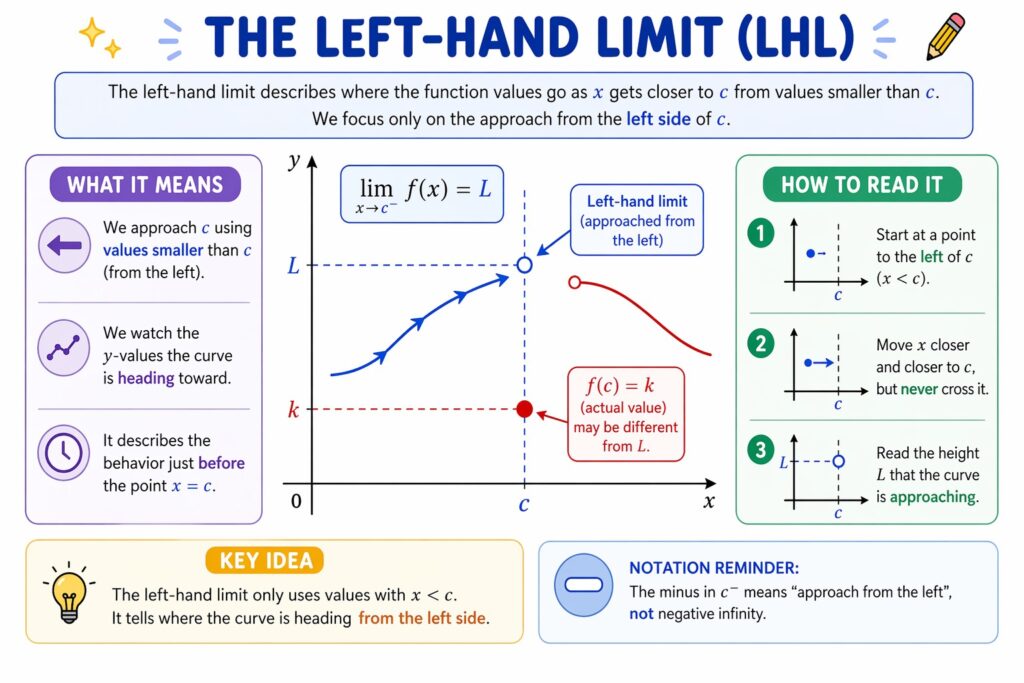
It also distinguishes the approached height from the actual function value at the point.
The Right-Hand Limit (RHL)
A right-hand limit examines the function's trend as the input approaches a value from the right. We focus on values that are slightly larger than the target. This perspective is crucial for identifying how a function starts after a specific point.
We denote this limit using a superscript plus sign. The notation ##\lim_{x \to c^+} f(x)## indicates that ##x## is getting closer to ##c## from the right. It represents the behavior of the function coming from the positive direction of the axis.
This method helps mathematicians define the behavior of piecewise functions at their boundaries. By looking at the right side, we can see if the function connects smoothly or if there is a gap. It provides a complete view of the point.
To find the RHL algebraically, you evaluate the function for values just above the target. You observe if the outputs settle on a specific numerical value. This is often done by substituting ##c + h## where ##h## is very small.
On a coordinate plane, you move your eyes along the graph from right to left. You stop at the target value to see the height reached. This height is the RHL, regardless of whether the point itself is filled or empty.
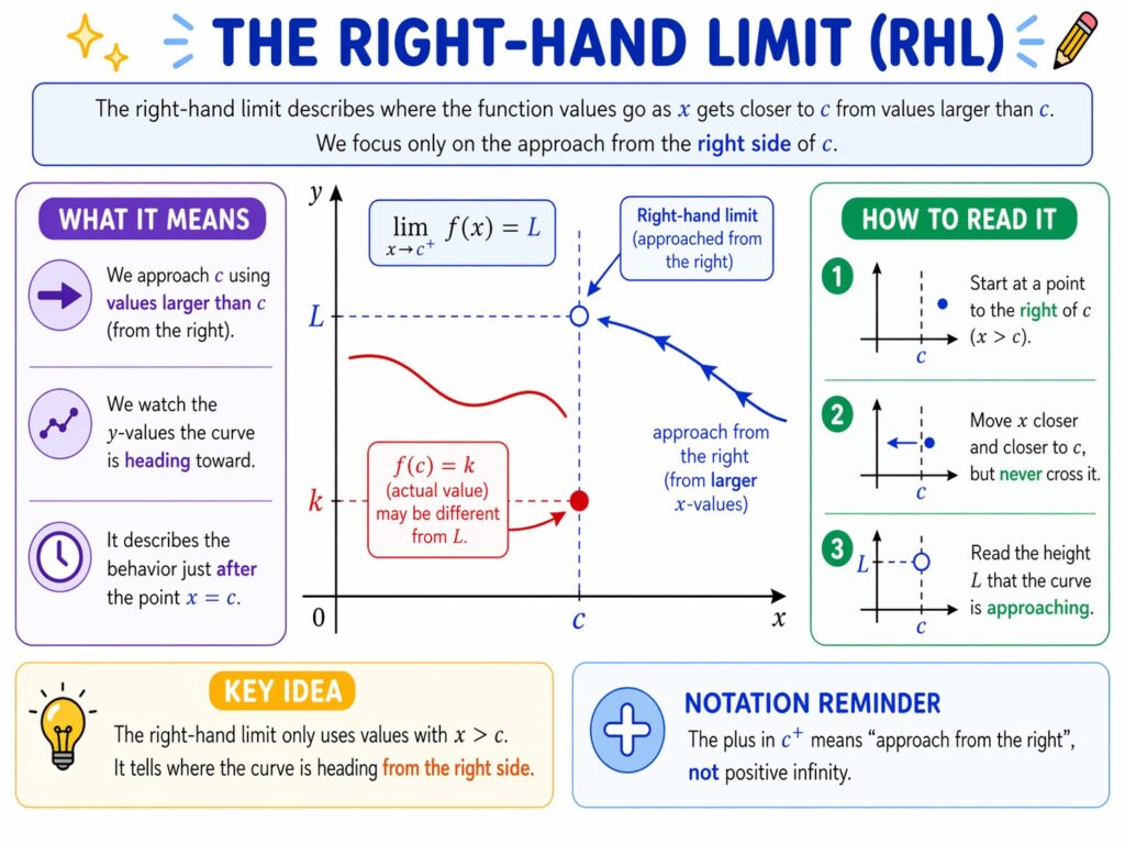
It also distinguishes the approached height from the actual function value at the point.
Conditions for Limit Existence
Equality of LHL and RHL
For a general limit to exist at a point, the left-hand and right-hand limits must match. They must point to the same numerical output value. This agreement ensures the function is heading toward a single point from both directions on the graph.
If the LHL is ##L## and the RHL is also ##L##, then the limit exists. We simply say the limit of the function at that point is ##L##. This is the most basic requirement for defining a limit in standard calculus courses.
If these two values differ, the general limit does not exist. This often happens at points where the graph has a vertical gap or jump. In such cases, we say the limit is undefined or simply write "DNE" for the answer.
Mathematical consistency requires this agreement from both directions. Without it, the function's behavior at that specific point is considered ambiguous. This rule helps maintain logic when we move into more advanced topics like continuity and derivatives in mathematics.
Math Problem 1:
To solve this, calculate the LHL using ##3x - 1## and the RHL using ##x + 1## at ##x = 1##. Since ##3(1)-1 = 2## and ##1+1 = 2##, the limit exists and equals ##2##.
Finite Value Requirement
A limit exists only if the function approaches a finite, real number. If the values of the function grow without bound, the limit is said to be infinite. While we use infinity symbols, the limit technically does not exist as a number.
Sometimes, a function oscillates rapidly as it approaches a point. If the values do not settle on one number, the limit does not exist. This is common in certain trigonometric functions where the frequency increases near zero or other specific points.
We must distinguish between a limit being infinite and a limit not existing due to disagreement. An infinite limit tells us about the growth rate, while a disagreement tells us about a break in the graph. Both are important for analysis.
In simple English, a limit is like a destination. If two people walking from different directions arrive at the same house, the destination exists. If they arrive at different houses or walk forever, there is no single shared destination point.
Calculus students must check both the direction and the finiteness of the result. If your calculations lead to ##\dfrac{1}{0}##, you are likely looking at an infinite limit. Always verify the behavior on both sides to be sure of the result.
Evaluating Piecewise Functions
Analyzing Jump Discontinuities
A jump discontinuity occurs when the LHL and RHL are both finite but not equal. The graph literally jumps from one height to another at a point. This is a classic example of where a two-sided limit fails to exist.
These breaks are common in step functions and piecewise-defined models. They represent sudden changes in the state of a system. For example, a tax bracket might jump at a certain income level, creating a clear discontinuity in the graph.
When you encounter a jump, the two-sided limit is labeled as "Does Not Exist". However, the individual one-sided limits still provide useful information. They tell us the starting and ending heights of the jump at that specific input value.
Identifying these jumps is a key skill in calculus. It helps in determining where a function is continuous. If you cannot draw the graph without lifting your pencil, you are likely dealing with a jump or another type of discontinuity.
Math Problem 2:
For ##x < 0##, ##f(x) = -1##, so LHL is ##-1##. For ##x > 0##, ##f(x) = 1##, so RHL is ##1##. Since ##-1 \neq 1##, the limit does not exist at ##x = 0##.
Practical Step-by-Step Evaluation
To evaluate a limit at a point ##a##, first identify the function's formula on the left side. Substitute values slightly smaller than ##a## to find the LHL. Write this value down clearly so you can compare it later in the process.
Next, identify the formula used on the right side of ##a##. Substitute values slightly larger than ##a## to determine the RHL. Ensure your arithmetic is correct, as even a small error can lead to the wrong conclusion about existence.
Compare the two results you obtained. If they are identical, that number is your final answer for the limit. If they are different, state that the limit does not exist. This simple comparison is the heart of limit evaluation.
Always check if the function is defined at the point itself. While the limit doesn't care about the actual value at ##a##, knowing it helps you understand continuity. A limit can exist even if the point is missing from the graph.
Use algebraic simplification if the direct substitution leads to an indeterminate form. Factoring or rationalizing can often reveal the hidden limit value. However, always apply these techniques to both the left and right sides if the function is piecewise.
Mathematical Notation and Symbols
Interpreting the Plus and Minus Signs
The symbols ##+## and ##-## in limit notation are not about the sign of the number. Instead, they indicate the direction of approach. A ##2^-## means "approaching 2 from the left," which includes values like ##1.9## and ##1.99##.
Similarly, ##2^+## means "approaching 2 from the right." This includes values like ##2.1## and ##2.01##. It is a common mistake for beginners to think these symbols mean negative or positive numbers. Always remember they represent the side of the approach.
When the notation has no sign, like ##\lim_{x \to 2}##, it implies a two-sided limit. You are required to check both sides automatically. If the problem doesn't specify a side, the answer depends on the agreement of both directions.
Using these symbols correctly makes your mathematical communication clear. It tells other mathematicians exactly which part of the function you are analyzing. This precision is what makes calculus a powerful tool for science and engineering fields worldwide.
In textbooks, you might see these called one-sided limits. They are the building blocks for more complex definitions. Mastering the notation is the first step toward solving difficult problems involving limits at infinity or vertical asymptotes in graphs.
Formal Definition of Existence
The formal definition states that ##\lim_{x \to a} f(x) = L## if and only if both one-sided limits equal ##L##. This is a biconditional requirement. It means the existence of the limit depends entirely on the behavior from both sides.
This rule ensures that the function approaches a single, predictable value. It creates a solid foundation for further operations like differentiation. If a function is "well-behaved" at a point, its left and right limits will always be the same.
If either one-sided limit is infinite, the general limit is often considered non-existent. We must specify the direction of the infinity to be accurate. For example, we might say the limit is positive infinity if both sides go up.
Understanding these conditions prevents errors in complex calculus problems. It forces a rigorous check of the function's behavior around critical points. Professional mathematicians always verify these conditions before assuming a limit exists in their proofs or calculations.
Math Problem 3:
Check the LHL : ##\lim_{x \to 3^-} x^2 = 3^2 = 9##
Check the RHL : ##\lim_{x \to 3^+} (2x + 3) = 2(3) + 3 = 9##
Since LHL = RHL = 9, the limit exists and is ##9##.
Test Your Understanding
Q1. Consider the piecewise function ##f(x)## defined as ##f(x) = 2x + 3## for ##x < 2## and ##f(x) = x^2 + 3## for ##x \geq 2##. Evaluate ##\lim_{x \to 2^-} f(x)##.
To find the left-hand limit as ##x \to 2^-##, we use the piece of the function where ##x < 2##. Substituting ##x = 2## into ##2x + 3## gives ##2(2) + 3 = 7##.
Q2. Determine the value of ##\lim_{x \to 4^+} \frac{\lvert x - 4 \rvert}{x - 4}##.
When ##x \to 4^+##, ##x > 4##, which means ##x - 4 > 0##. Therefore, ##\lvert x - 4 \rvert = x - 4##. The expression becomes ##\frac{x - 4}{x - 4} = 1##.
Q3. Find the right-hand limit ##\lim_{x \to 0^+} \frac{5}{x}##.
As ##x## approaches ##0## from the right, ##x## is a very small positive number. Dividing a positive constant ##5## by a vanishingly small positive number results in a value that grows without bound toward ##\infty##.
Q4. Let ##f(x) = \lfloor x \rfloor## be the greatest integer function (floor function). What is the value of ##\lim_{x \to 3^-} (x + \lfloor x \rfloor)##?
As ##x \to 3^-##, ##x## is slightly less than 3 (e.g., 2.99). The greatest integer less than or equal to 2.99 is ##\lfloor 2.99 \rfloor = 2##. The limit becomes ##3 + 2 = 5##.
Q5. For what value of the constant ##k## does ##\lim_{x \to 1} f(x)## exist, if ##f(x) = kx + 2## for ##x < 1## and ##f(x) = x^2 - k## for ##x \geq 1##?
For the limit to exist, LHL must equal RHL. LHL (as ##x \to 1^-##) is ##k(1) + 2 = k + 2##. RHL (as ##x \to 1^+##) is ##1^2 - k = 1 - k##. Setting them equal: ##k + 2 = 1 - k \Rightarrow 2k = -1 \Rightarrow k = -0.5##.
Q6. Evaluate ##\lim_{x \to 0^-} \frac{\sqrt{x^2}}{x}##.
Note that ##\sqrt{x^2} = \lvert x \rvert##. As ##x \to 0^-##, ##x## is negative, so ##\lvert x \rvert = -x##. The expression simplifies to ##\frac{-x}{x} = -1##.
Q7. If ##\lim_{x \to c^-} f(x) = L_1## and ##\lim_{x \to c^+} f(x) = L_2##, under which condition can we say ##\lim_{x \to c} f(x)## exists?
The definition of a limit existing at a point ##c## requires that the left-hand limit and right-hand limit are equal and finite. The value of the function at ##c##, ##f(c)##, is relevant for continuity but not for the existence of the limit itself.
Q8. Consider the function ##f(x) = \frac{1}{x - 5}##. Which of the following statements is true regarding its one-sided limits at ##x = 5##?
As ##x \to 5^-##, ##x - 5## is a small negative number, so ##\frac{1}{x-5} \to -\infty##. As ##x \to 5^+##, ##x - 5## is a small positive number, so ##\frac{1}{x-5} \to \infty##.
Q9. Evaluate ##\lim_{x \to 2^+} \frac{x^2 - 4}{\lvert x - 2 \rvert}##.
First, factor the numerator: ##x^2 - 4 = (x-2)(x+2)##. Since ##x \to 2^+##, ##x > 2##, so ##\lvert x - 2 \rvert = x - 2##. The expression becomes ##\frac{(x-2)(x+2)}{x-2} = x + 2##. Substituting ##x = 2## gives ##2 + 2 = 4##.
Q10. What is ##\lim_{x \to 0^+} e^{-1/x}##?
As ##x \to 0^+##, the exponent ##-1/x \to -\infty##. The function ##e^u## approaches ##0## as ##u \to -\infty##. Therefore, the limit is ##0##.
RESOURCES
- Master Left-Hand & Right-Hand Limits in Calculus - YouTube
- Left and Right-Hand Limits
- How to find the left and right hand limit by not using a calculator
- Calculus I - One-Sided Limits - Pauls Online Math Notes
- Lesson 12 - Left Hand And Right Hand Limits, Part 2 (Calculus 1)
- left and right hand limits - Mathematics Stack Exchange
- One-sided limit - Wikipedia
- When to know to use or to check left and right-hand limit ... - Reddit
- How to determine the Left and Right limit of a function - Free Math Help
- Calculating right/left hand limits : r/MathHelp - Reddit
- If both the left and right hand limits approach positive infinity, does ...
- Left Hand & Right Hand Limits: Definition, Diagram, Solved ...
- One-Sided Limits with Solved Example - GeeksforGeeks
- Symbols for left and right limits - TeX - LaTeX Stack Exchange
- 1.4: One Sided Limits - Mathematics LibreTexts
0 Comments