What Are Isotopes? Nuclear Variants, Stability, and Their Scientific Reach

Isotopes are among the most consequential ideas in all of physical science, yet the term is often reduced to a single line in a textbook: atoms of the same element with different numbers of neutrons. That definition is correct, but it conceals an extraordinary depth. Every isotope carries a distinct nuclear signature, a specific mass, a characteristic stability, and often a unique behaviour that ripples outward into chemistry, medicine, geology, and astrophysics. Understanding isotopes means understanding why the periodic table is not a flat catalogue of elements but a layered architecture of nuclear variants, each with its own story.

The concept reshaped how scientists think about the atom itself. When Frederick Soddy proposed the term in 1913 to explain chemically identical substances with different radioactive behaviour, he was describing something that seemed almost paradoxical: two atoms that behave identically in every chemical reaction yet decay at completely different rates. That paradox resolved into the modern picture of a nucleus built from protons and neutrons, where the proton count defines the element and the neutron count defines the isotope. The consequences of that simple distinction are enormous, reaching from the calibration of medical imaging devices to the dating of the oldest rocks on Earth.

This analysis examines isotopes through their definition, their notation, their physical origins, their stability patterns, their analytical measurement, and their practical applications across the sciences. It treats the topic with the mathematical rigour the subject deserves, including the governing equations for isotopic abundance, radioactive decay, and mass spectrometry, while keeping the narrative grounded in the physical reality of what these nuclear variants actually are and why they matter so profoundly.

The Nuclear Definition and Atomic Architecture of Isotopes

An isotope is a variant of a chemical element defined by a specific number of neutrons in its atomic nucleus while retaining the same number of protons. Because the proton count, known as the atomic number ##[Z]##, determines the element's chemical identity, all isotopes of a given element occupy the same position in the periodic table and share nearly identical electronic configurations. The neutron count ##[N]## varies, and the sum ##[A = Z + N]## gives the mass number, which distinguishes one isotope from another.

Protons, Neutrons, and the Mass Number

The nucleus sits at the centre of the isotope concept. Protons carry positive charge and establish the electrostatic environment that binds electrons into shells, while neutrons contribute mass and, crucially, the strong nuclear force that counteracts proton-proton repulsion. Adding or removing a neutron changes the mass and the nuclear binding energy without altering the charge, which is precisely why isotopes of an element are chemically almost indistinguishable yet physically distinct.

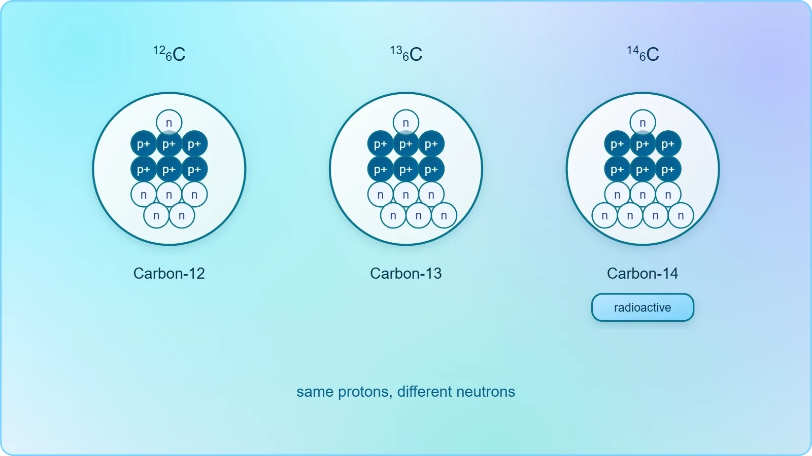
Consider carbon, the backbone of organic chemistry. Its nucleus always contains six protons, but the neutron count can be six, seven, or eight, yielding carbon-12, carbon-13, and carbon-14 respectively. Carbon-12 and carbon-13 are stable, while carbon-14 is radioactive with a half-life of roughly 5,730 years. The mass number ##[A]## is written as a superscript before the symbol, so carbon-14 appears as ##[^{14}_{6}\text{C}]##, where the subscript denotes the atomic number and the superscript the mass number.

The mass of an isotope is not simply the sum of its constituent particle masses, because a portion of that mass is converted into nuclear binding energy according to ##[E = mc^2]##. This mass defect is small but measurable, and it explains why the atomic mass of an isotope differs slightly from the integer mass number. The difference, called the mass excess, is a fundamental quantity in nuclear physics and underpins techniques such as mass spectrometry.

Isotopes also differ in their spin and magnetic properties, which arise from the arrangement of unpaired nucleons. These nuclear spin states are the basis of nuclear magnetic resonance spectroscopy, a technique that has become indispensable in chemistry and medicine. Thus the neutron count does not merely add mass; it reshapes the quantum state of the entire nucleus and, through hyperfine interactions, can subtly influence atomic spectra.

Isobars, Isotones, and Nuclear Neighbours

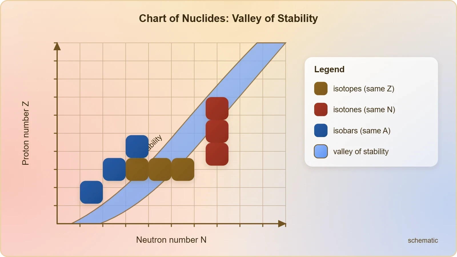
The vocabulary of nuclear variants extends beyond isotopes. Isobars are nuclides with the same mass number ##[A]## but different proton counts, such as argon-40 and calcium-40. Isotones share the same neutron number ##[N]##, for example carbon-13 and nitrogen-14, each with seven neutrons. These categories matter because nuclear stability depends on the interplay between ##[Z]## and ##[N]##, and neighbouring nuclides often transform into one another through decay.

The distinction between isotopes and isobars is not merely semantic. Isobars of the same mass number can interconvert through beta decay, where a neutron transforms into a proton or vice versa, changing the element entirely. This is why the decay chains of heavy elements produce a cascade of different elements, each step shifting the proton count while preserving the total nucleon number in the parent nucleus.

Isotones are particularly useful in nuclear shell theory, where magic neutron numbers such as 50, 82, and 126 confer exceptional stability. A nucleus with a magic neutron count behaves like a closed shell, analogous to the noble gas configuration in electron shells. This parallel between nuclear and electronic shell structure is one of the most elegant unifications in modern physics.

Understanding these neighbouring categories helps clarify why the chart of nuclides is a two-dimensional map rather than a simple list. Each nuclide occupies a coordinate defined by ##[Z]## and ##[N]##, and the patterns of stability, decay, and synthesis trace out structures that reveal the underlying nuclear forces at work.

Notation, Atomic Mass, and the Mathematics of Abundance

Isotopic notation provides a compact language for describing nuclear composition, and the mathematics of isotopic abundance connects the microscopic world of individual nuclei to the macroscopic measurements chemists make in the laboratory. The atomic weight printed on the periodic table is not the mass of a single atom but a weighted average over all naturally occurring isotopes, and that averaging process is governed by a simple but powerful formula.

Reading Isotopic Symbols and Mass Spectra

The standard notation places the mass number as a superscript and the atomic number as a subscript before the element symbol, as in ##[^{235}_{92}\text{U}]## for uranium-235. Sometimes the mass number alone suffices, written as uranium-235 or U-235. In mass spectrometry, the output is a spectrum of peaks, each corresponding to an isotope or fragment, with peak height proportional to abundance and peak position determined by the mass-to-charge ratio ##[m/z]##.

Mass spectrometry exploits the fact that ions moving through electric and magnetic fields follow trajectories that depend on their mass-to-charge ratio. The governing relation for a charged particle in a magnetic field is the Lorentz force, which curves the path with a radius given by the momentum divided by the product of charge and field strength. Lighter isotopes curve more sharply, allowing physical separation and precise abundance measurement.

The resolving power of a mass spectrometer determines how closely spaced isotopes can be distinguished. High-resolution instruments can separate isotopes differing by a single neutron, and even by the small mass defect differences between isobars. This capability is essential in fields ranging from environmental monitoring to forensic analysis, where isotopic fingerprints can identify the origin of a sample.

Isotopic symbols also appear in nuclear reaction equations, where conservation of mass number and atomic number must hold on both sides. Balancing such equations is a routine exercise in nuclear chemistry, and it reinforces the fundamental principle that nucleons are conserved in ordinary nuclear transformations, even as elements transmute into one another.

Calculating Average Atomic Mass

The average atomic mass of an element is the abundance-weighted mean of its isotope masses. If an element has isotopes with masses ##[m_i]## and fractional abundances ##[f_i]##, the average mass is given by the summation over all isotopes. This formula is the bridge between the discrete nuclear world and the continuous measurements of bulk chemistry.

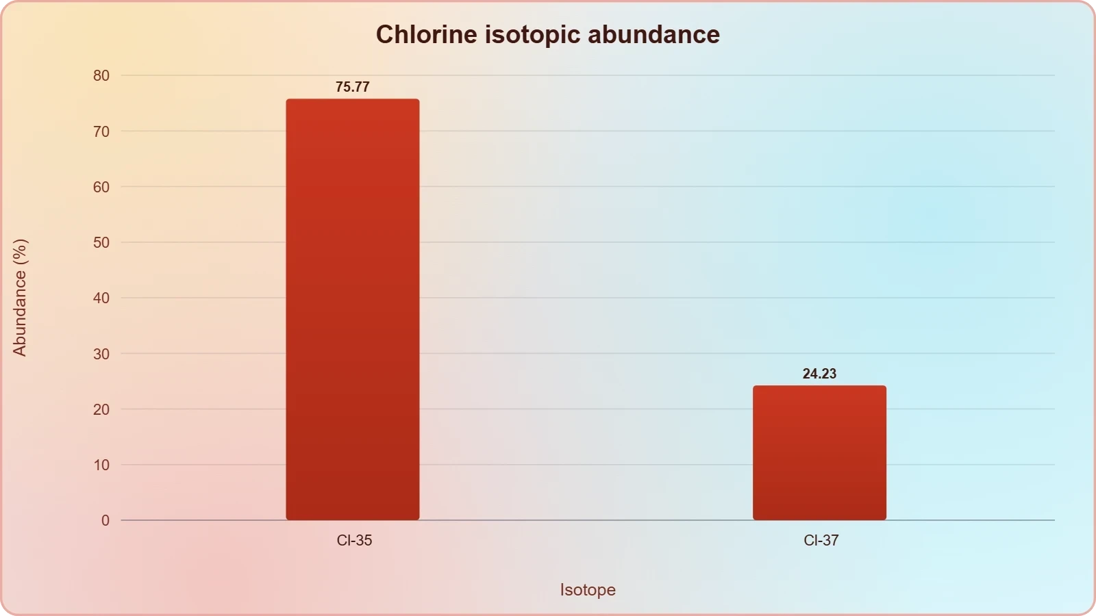
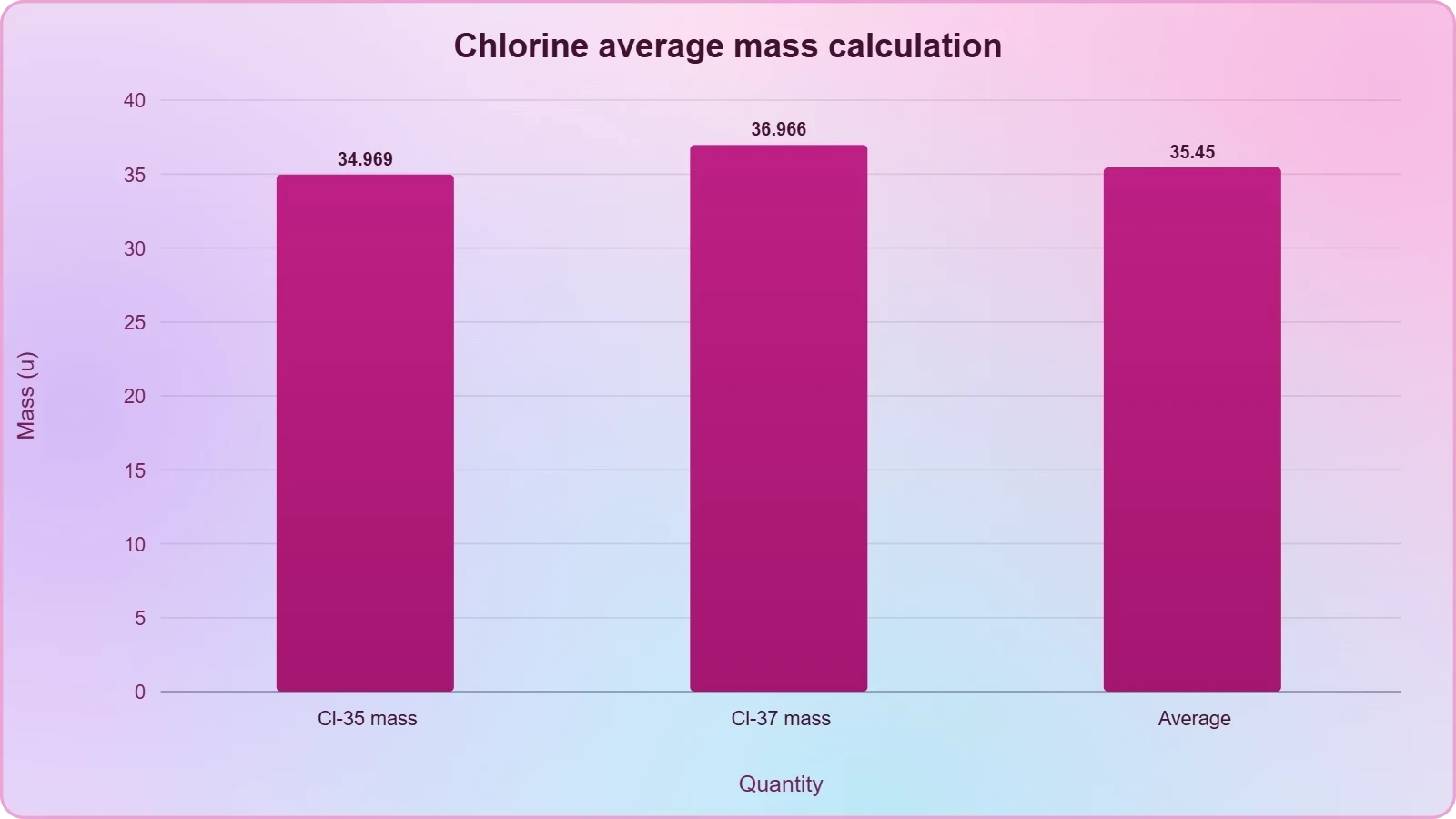
Chlorine provides a classic illustration. Naturally occurring chlorine consists of approximately 75.77 percent chlorine-35 and 24.23 percent chlorine-37. Applying the weighted average formula yields an atomic mass close to 35.45 atomic mass units, which matches the value on the periodic table. The calculation demonstrates how a non-integer atomic weight arises from a mixture of integer-mass isotopes.

Fractional abundances are usually expressed as percentages but must be converted to decimals before substitution. A common error is to forget this conversion, which inflates the result by a factor of one hundred. Careful dimensional reasoning and unit tracking prevent such mistakes, and they reinforce the habit of checking that the final mass lies between the lightest and heaviest isotope masses.

Isotopic abundance is not fixed across the universe. Meteorites, for example, can show slight enrichments or depletions relative to terrestrial samples, and these anomalies carry information about the conditions in the early solar system. Measuring such variations requires extremely precise mass spectrometry and provides a window into astrophysical processes that occurred billions of years ago.

Nuclear Stability, Binding Energy, and Radioactive Decay

Not every combination of protons and neutrons produces a stable nucleus. The chart of nuclides reveals a narrow band of stability, often called the valley of stability, where the balance between the strong nuclear force and electrostatic repulsion allows a nucleus to persist indefinitely. Isotopes outside this band are radioactive and transform toward stability through various decay modes, each governed by precise mathematical laws.

The Valley of Stability and Binding Energy

Nuclear binding energy is the energy required to disassemble a nucleus into its constituent protons and neutrons. It arises from the mass defect, the difference between the sum of free nucleon masses and the actual nuclear mass. The binding energy per nucleon peaks near iron-56, which is why iron sits at the endpoint of stellar fusion and why both lighter and heavier nuclei can release energy through fusion or fission respectively.

For light nuclei, the neutron-to-proton ratio is close to one, and stability requires roughly equal numbers of each. As nuclei grow heavier, electrostatic repulsion among protons increases, and additional neutrons are needed to provide sufficient strong-force attraction without adding charge. This is why heavy stable nuclei have neutron-to-proton ratios approaching 1.5, and why uranium-238, with 92 protons and 146 neutrons, is only weakly stable.

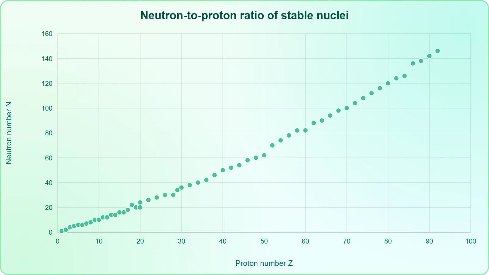
Magic numbers add another layer of structure. Nuclei with proton or neutron counts equal to 2, 8, 20, 28, 50, 82, or 126 exhibit enhanced stability, analogous to closed electron shells. Doubly magic nuclei, such as helium-4 with two protons and two neutrons, are exceptionally tightly bound. These patterns emerge from the nuclear shell model and provide a quantum mechanical explanation for the observed stability landscape.

Beyond the valley of stability lie thousands of known radionuclides, many produced artificially in reactors and accelerators. Some have half-lives measured in fractions of a second, while others persist for millions of years. Mapping this territory is an active area of nuclear physics, with implications for understanding stellar nucleosynthesis and for designing new medical and industrial isotopes.

Decay Kinetics and Half-Life Mathematics

Radioactive decay is a stochastic process at the level of individual nuclei, but it follows a precise exponential law in aggregate. The number of undecayed nuclei decreases according to a first-order differential equation, whose solution introduces the decay constant ##[\lambda]## and the half-life ##[t_{1/2}]##. These quantities are related by a simple logarithmic expression that appears throughout nuclear science.

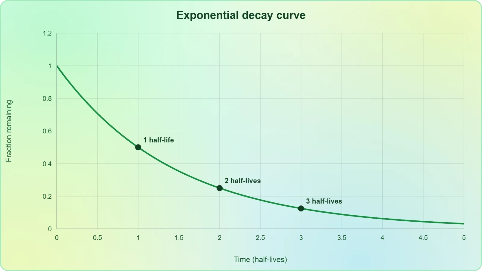
The activity of a sample, defined as the number of decays per unit time, is proportional to the number of undecayed nuclei and the decay constant. This relationship underlies radiometric dating, medical dosimetry, and the management of nuclear waste. Because activity decreases exponentially, a sample's age can be inferred from the ratio of parent to daughter isotopes, provided the initial conditions are known.

Different decay modes dominate in different regions of the chart of nuclides. Alpha decay is common among heavy nuclei, beta decay occurs when the neutron-to-proton ratio is unbalanced, and gamma emission accompanies transitions between excited nuclear states. Each mode has its own selection rules and energy spectrum, and together they provide a rich diagnostic toolkit for identifying unknown isotopes.

Carbon-14 dating illustrates the power of decay kinetics in practice. Living organisms continuously exchange carbon with their environment, maintaining a steady carbon-14 level. Once an organism dies, the carbon-14 decays without replenishment, and the remaining fraction reveals the time elapsed since death. The method has transformed archaeology and palaeontology, though its range is limited to roughly fifty thousand years.

Separation, Enrichment, and Analytical Measurement

Because isotopes of an element are chemically nearly identical, separating them is a formidable technical challenge. The small mass differences that distinguish isotopes provide the only practical handle, and every separation method exploits some mass-dependent physical process. Enrichment technology is therefore a study in precision engineering, with applications ranging from nuclear fuel production to the preparation of stable isotope tracers for medical research.

Physical Separation Techniques

Gaseous diffusion relies on the slightly higher average speed of lighter molecules. Uranium hexafluoride containing uranium-235 diffuses through a porous barrier marginally faster than the uranium-238 variant, and repeated stages amplify the tiny enrichment achieved per pass. The process is energy-intensive, which is why modern facilities increasingly favour gas centrifugation instead.

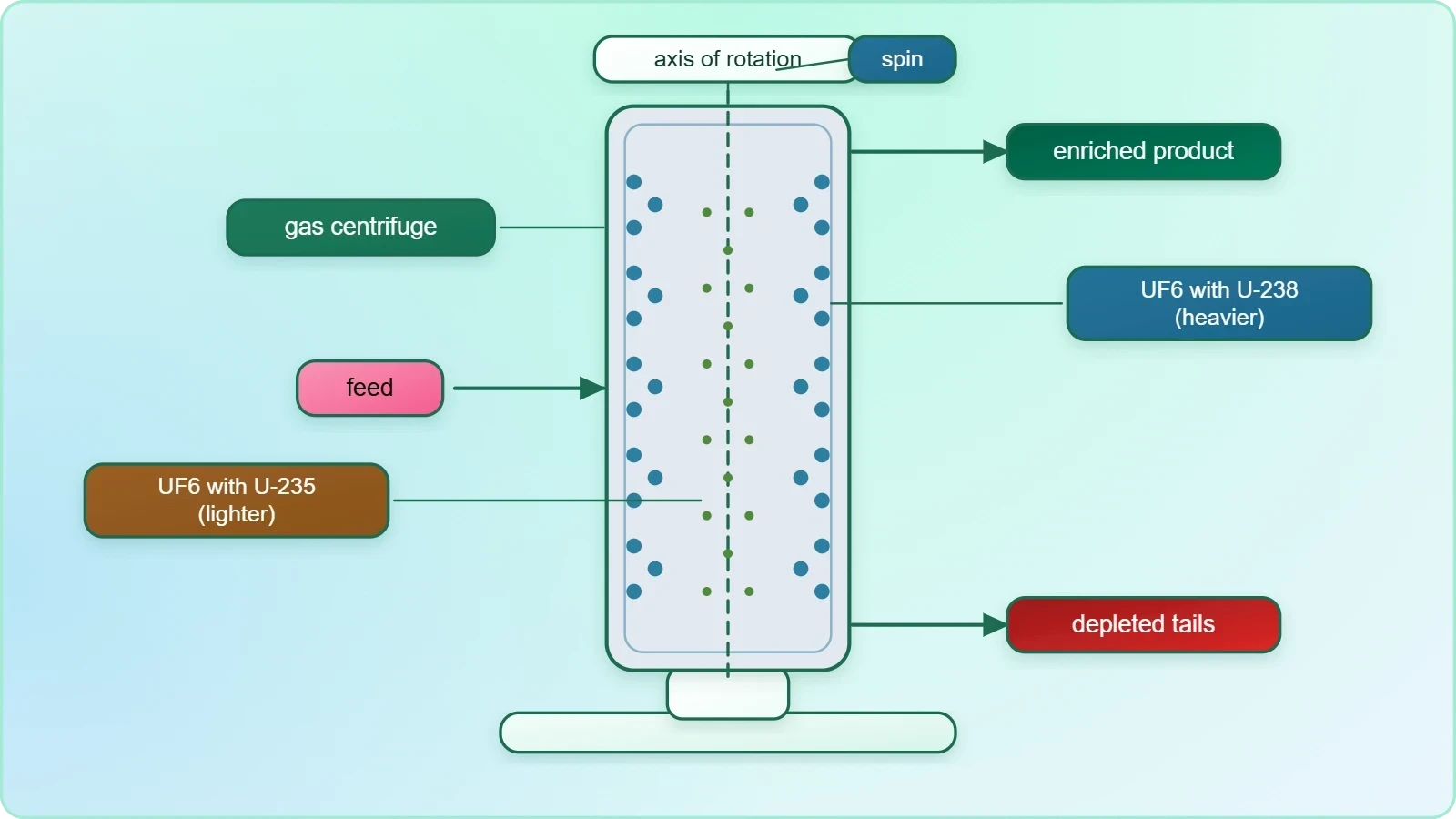
Gas centrifugation spins uranium hexafluoride at high speed, causing heavier molecules to concentrate near the outer wall while lighter ones remain closer to the axis. A single centrifuge achieves modest separation, but cascades of thousands of units can produce highly enriched uranium. The physics is elegant, but the engineering demands extreme precision and materials capable of withstanding enormous centrifugal stress.

Other methods include electromagnetic separation, laser isotope separation, and chemical exchange. Laser separation exploits tiny differences in atomic energy levels between isotopes, allowing selective ionisation and collection. Each technique has trade-offs in cost, throughput, and selectivity, and the choice depends on the intended application and the scale of production required.

Stable isotope separation serves a different purpose. Isotopes such as carbon-13, nitrogen-15, and deuterium are valuable tracers in metabolic studies, nuclear magnetic resonance, and mass spectrometry. Producing them requires similar separation principles but at smaller scale, and the resulting enriched compounds command high prices in research markets.

Mass Spectrometry and Isotopic Fingerprinting

Mass spectrometry is the workhorse of isotopic analysis. A sample is ionised, accelerated, and separated according to mass-to-charge ratio, producing a spectrum whose peaks reveal the isotopic composition. Modern instruments achieve extraordinary sensitivity, detecting isotopes at parts-per-trillion levels and resolving mass differences smaller than a single electron mass.

Isotope ratio mass spectrometry extends this capability to precise abundance measurements, enabling applications in climate science, forensics, and food authentication. The ratio of carbon-13 to carbon-12, for example, can reveal whether a food product was derived from a C3 or C4 plant, exposing adulteration in honey, juice, and vanilla. Such applications demonstrate how nuclear-level measurements inform everyday commerce.

Accelerator mass spectrometry pushes sensitivity further by counting individual atoms of rare isotopes. It is the method of choice for radiocarbon dating, where carbon-14 atoms are exceedingly scarce, and for detecting trace radionuclides in environmental samples. The technique combines particle acceleration with sophisticated detection, achieving detection limits that conventional mass spectrometry cannot approach.

Isotopic fingerprinting also has forensic value. The isotopic composition of hair, teeth, and bones reflects diet and geography, allowing investigators to trace human remains or verify the provenance of materials. This application rests on the subtle natural variations in isotopic abundance that arise from climatic and geological processes, and it illustrates how the smallest nuclear differences can carry substantial information.

Applications Across Medicine, Geology, and Energy

The practical reach of isotope science is remarkably broad. Medical imaging, cancer therapy, geological dating, environmental tracing, and nuclear energy all depend on the distinctive properties of specific isotopes. Each application exploits a different aspect of nuclear behaviour, whether it is the emission of radiation, the rate of decay, or the subtle mass differences that allow isotopes to be tracked through complex systems.

Medical Imaging and Targeted Therapy

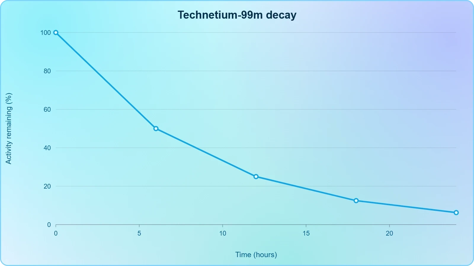
Technetium-99m is the most widely used medical radioisotope, employed in tens of millions of diagnostic procedures annually. Its short half-life of six hours and its emission of gamma rays make it ideal for single-photon emission computed tomography, allowing clinicians to image organ function with minimal radiation dose to the patient. The isotope is generated on-site from a molybdenum-99 parent.

Positron emission tomography relies on isotopes such as fluorine-18, which decays by positron emission. The annihilation of the positron with an electron produces two gamma photons travelling in opposite directions, and detecting these coincident photons allows precise localisation of the tracer within the body. Fluorodeoxyglucose labelled with fluorine-18 is used extensively in oncology to identify metabolically active tumours.

Therapeutic isotopes exploit the damaging effects of radiation on diseased tissue. Iodine-131 concentrates in the thyroid and is used to treat hyperthyroidism and thyroid cancer. Lutetium-177, coupled to targeting peptides, delivers radiation directly to neuroendocrine tumours. These targeted radionuclide therapies represent a growing frontier in precision oncology, where the isotope becomes a guided weapon against malignant cells.

Stable isotopes also contribute to medicine. Deuterated drugs, in which hydrogen atoms are replaced by deuterium, can exhibit altered metabolic stability and improved pharmacokinetics. The heavier isotope slows certain metabolic reactions through the kinetic isotope effect, extending drug half-life and reducing dosing frequency. Several deuterated pharmaceuticals have reached the market, validating this subtle application of nuclear mass differences.

Geochronology, Tracers, and Nuclear Energy

Radiometric dating depends on the decay of long-lived isotopes. Uranium-lead dating, using the decay of uranium-238 to lead-206 and uranium-235 to lead-207, has established the age of the Earth at approximately 4.54 billion years. Potassium-argon and rubidium-strontium methods extend the technique to different time ranges and materials, providing a comprehensive chronology of geological and archaeological events.

Isotopes serve as tracers in environmental science, hydrology, and ecology. The ratio of oxygen-18 to oxygen-16 in ice cores records past temperatures, providing a detailed archive of climate history. Nitrogen-15 tracing reveals nutrient cycling in ecosystems, while strontium isotopes fingerprint the migration patterns of ancient peoples and animals. These applications transform isotopes into natural labels that reveal processes invisible to direct observation.

Nuclear energy depends on the fission of uranium-235, whose ability to sustain a chain reaction stems from its nuclear properties. The fission of one uranium-235 nucleus releases approximately 200 MeV of energy, vastly exceeding chemical combustion. Controlled chain reactions in reactors and uncontrolled reactions in weapons both exploit the same fundamental physics, which is why isotope enrichment is a matter of international security concern.

Emerging applications continue to expand the isotope horizon. Isotope-based batteries, isotopic power sources for deep-space probes, and isotope-selective catalysis are active research areas. Each builds on the same foundational understanding: that the neutron count of a nucleus, though invisible to chemistry, shapes the physical behaviour of matter in ways that science continues to harness.

Worked Problems in Isotopic Calculation

Mastering isotopes requires fluency with the numerical relationships that connect nuclear composition to measurable quantities. The following worked problems illustrate the core calculations: average atomic mass, decay kinetics, binding energy, and enrichment factors. Each problem is presented with its full derivation, and together they form a compact problem set that reinforces the conceptual material developed throughout this analysis.

Abundance and Mass Calculations

Problem 1. Calculate the average atomic mass of chlorine given chlorine-35 at 75.77 percent with mass 34.9689 u and chlorine-37 at 24.23 percent with mass 36.9659 u. Converting percentages to decimals and applying the weighted average formula gives the result below.

Problem 2. A sample of boron contains boron-10 at 19.9 percent and boron-11 at 80.1 percent. Given isotope masses of 10.0129 u and 11.0093 u, the average atomic mass follows directly from the same weighted sum, yielding approximately 10.811 u, consistent with the tabulated value.

Problem 3. Determine the fractional abundance of lithium-6 given that lithium-7 has a mass of 7.0160 u, lithium-6 has a mass of 6.0151 u, and the average atomic mass is 6.941 u. Let ##[x]## be the fraction of lithium-6 and solve the linear equation that results from the weighted average condition.

Decay and Energy Calculations

Problem 4. Carbon-14 has a half-life of 5,730 years. Calculate its decay constant using the relation between half-life and decay constant, then determine the fraction remaining after 10,000 years by evaluating the exponential decay law at the appropriate time.

Problem 5. A sample contains ##[2.0 \times 10^{12}]## atoms of a radioisotope with a half-life of 12.3 years. Compute the initial activity in becquerels by multiplying the atom count by the decay constant expressed in inverse seconds, then convert to curies if required.

Problem 6. Calculate the binding energy of helium-4 given a nuclear mass of 4.0015 u, a proton mass of 1.00728 u, and a neutron mass of 1.00867 u. The mass defect multiplied by the square of the speed of light yields the binding energy in joules, which can be converted to MeV.

Problem 7. Determine the binding energy per nucleon for the helium-4 nucleus from the previous result. Dividing the total binding energy by the mass number gives a value near 7.07 MeV per nucleon, which is exceptionally high for a light nucleus and explains helium-4's remarkable stability.

Problem 8. Uranium-238 decays to lead-206 with a half-life of 4.47 billion years. For a mineral sample in which the lead-206 to uranium-238 ratio is 0.75, determine the sample's age using the decay equation rearranged to solve for time in terms of the isotope ratio.

Problem 9. A gas centrifuge cascade enriches uranium from 0.72 percent to 3.5 percent uranium-235. If each stage provides a separation factor of 1.0043, estimate the number of stages required using the logarithmic ratio of enrichment factors, a standard approximation in enrichment cascade design.

Problem 10. The kinetic isotope effect for deuterium substitution can slow a reaction by a factor related to the square root of the mass ratio. Estimate the maximum primary kinetic isotope effect for replacing hydrogen with deuterium using the reduced-mass ratio, which yields a factor of approximately seven at room temperature.

These ten problems span the quantitative core of isotope science, from simple abundance averaging to cascade design and kinetic isotope effects. Working through them builds the numerical intuition that transforms a definition into a working understanding, and it prepares the reader to engage with more advanced topics in nuclear chemistry and physics.