Mendel's decision to follow two characters at once rather than one transformed inheritance from a curiosity into a predictive science. When he crossed a pea plant bearing yellow, round seeds with one bearing green, wrinkled seeds, the first filial generation came out uniformly yellow and round, confirming that yellow dominates green and round dominates wrinkled. That much was already familiar from monohybrid work. The genuinely new information lay in the second filial generation, where four phenotypic classes appeared in the celebrated 9:3:3:1 proportion. Crucially, the yellow-to-green ratio inside that generation remained 3:1, and the round-to-wrinkled ratio also remained 3:1, as though each character had been inherited in complete ignorance of the other.
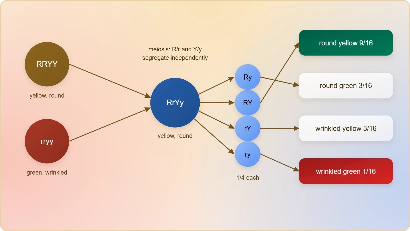
That observation is the heart of the Law of Independent Assortment, which states that when two pairs of traits are combined in a hybrid, the segregation of one pair of characters is independent of the other pair. The law does not merely describe a ratio; it asserts a mechanism, namely that the factors for different characters are distributed to gametes without reference to one another. Modern cytology explains why this works so well for genes on separate chromosomes, and equally explains why it fails for genes that travel together on the same chromosome. This lesson builds directly on the incomplete dominance and multiple allele complications examined previously, and it prepares the ground for the chromosomal theory and linkage that follow.
What follows is a working treatment rather than a summary. You will construct Punnett squares step by step, apply the product and sum rules to bypass tedious grid work, examine recombination frequency as the quantitative measure of independence, and confront the exceptions that forced geneticists to refine Mendel's second law. The 9:3:3:1 ratio will be derived three separate ways so that it becomes a tool you can manipulate rather than a number you memorise. By the end, the dihybrid cross should feel less like an exercise in filling sixteen boxes and more like a logical consequence of how chromosomes behave at meiosis.
On This Page
The Dihybrid Cross: Design, Symbols, and First Results
A dihybrid cross follows two pairs of contrasting traits simultaneously, and its design mirrors the monohybrid cross in every structural respect. Mendel selected seed colour, with yellow dominant over green, and seed shape, with round dominant over wrinkled. Using the genotypic symbols Y for yellow and y for green, R for round and r for wrinkled, the true-breeding parents are written RRYY and rryy. Each parent produces only one class of gamete, RY and ry respectively, so fertilisation yields the F1 hybrid RrYy without ambiguity. The choice of true-breeding parents matters enormously, because heterozygosity at either locus in the parental generation would obscure the clean deduction of gamete frequencies.
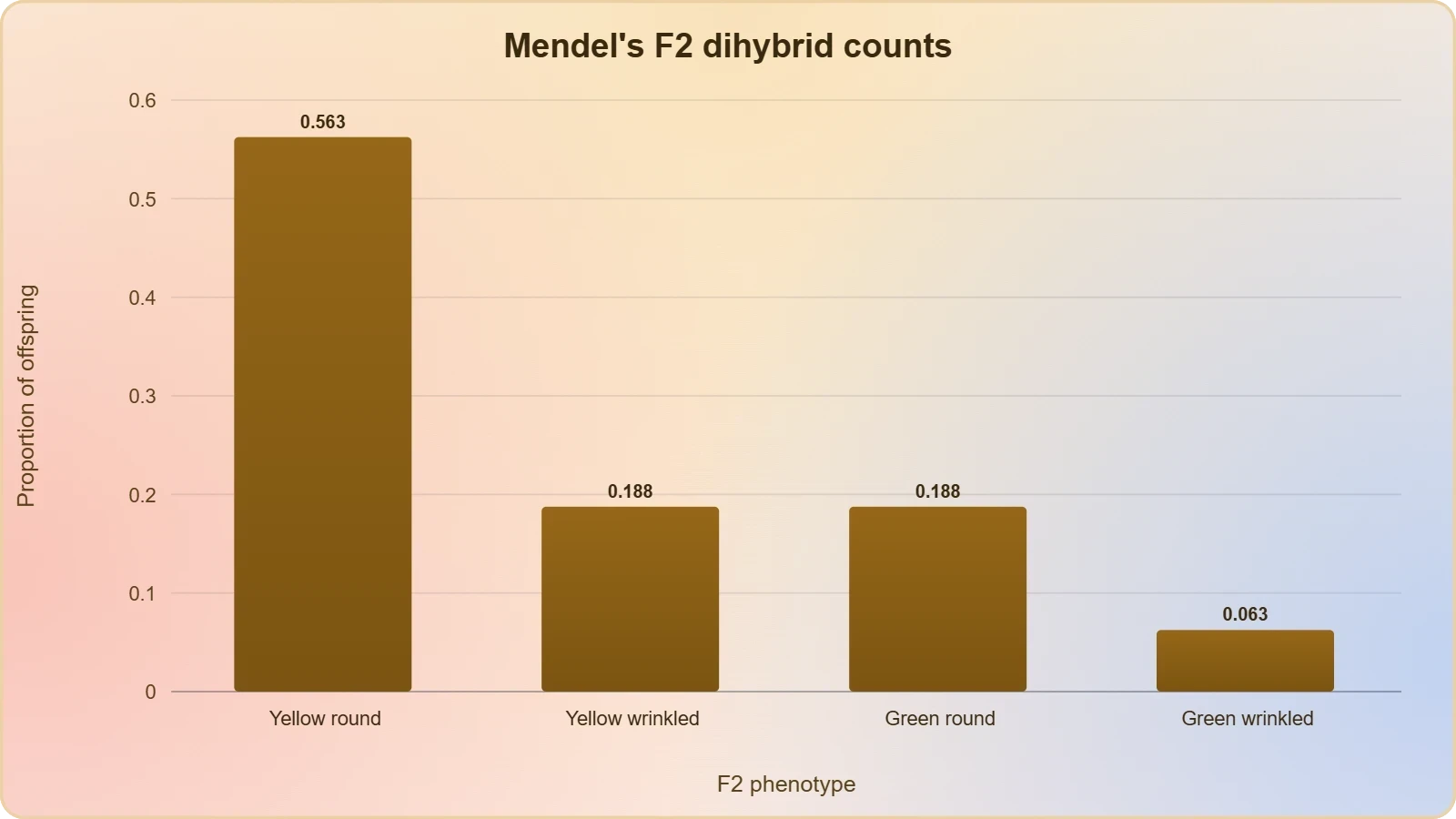
The F1 phenotype is yellow and round, which immediately establishes dominance at both loci. When Mendel self-hybridised these F1 plants, the F2 generation contained yellow round, yellow wrinkled, green round, and green wrinkled seeds. Counting the classes gave approximately nine, three, three, and one in every sixteen offspring. Equally important, when each character was scored in isolation, yellow to green came out 3:1 and round to wrinkled came out 3:1. The two monohybrid ratios had survived intact inside a two-character experiment, which is precisely the signature of independent behaviour.
Constructing the Sixteen-Square Punnett Grid
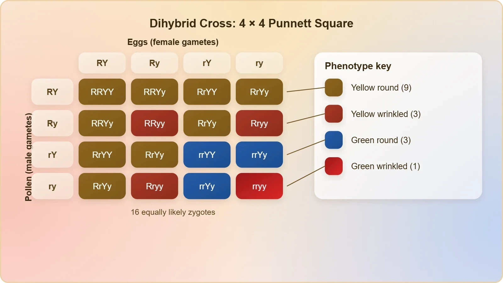
The Punnett square for a dihybrid cross begins with gamete enumeration. An RrYy plant produces four gamete genotypes, RY, Ry, rY, and ry, each at a frequency of one quarter, because the segregation of R from r is independent of the segregation of Y from y. Fifty per cent of gametes carry R and fifty per cent carry r; independently, fifty per cent carry Y and fifty per cent carry y. Combining these probabilities gives one quarter for each of the four combinations. Writing the four egg types along one axis and the four pollen types along the other produces a grid of sixteen cells, each representing an equally likely zygotic combination.
Reading the grid requires patience but no cleverness. Each cell receives one allele from the column header and one from the row header, conventionally written with the colour locus first. The cell at the intersection of RY eggs and rY pollen is RrYY, for instance, while Ry eggs with ry pollen give Rryy. Once all sixteen cells are filled, identical genotypes are pooled. The result is nine distinct genotypes and four distinct phenotypes. The phenotypic tally is nine round yellow, three round green, three wrinkled yellow, and one wrinkled green, which is the 9:3:3:1 ratio in its canonical form.
Deriving the Ratio Without the Grid
The sixteen-square grid is a teaching device, not a computational necessity. Because the two loci behave independently, the dihybrid outcome is the product of two monohybrid outcomes. Each character independently yields a 3:1 phenotypic ratio, so multiplying the two binomials gives the combined expectation. Written as a combination series, the derivation is compact and exact: (3 round : 1 wrinkled) multiplied by (3 yellow : 1 green) yields 9 round yellow, 3 round green, 3 wrinkled yellow, and 1 wrinkled green. The arithmetic of expanding two binomials is all that is required.
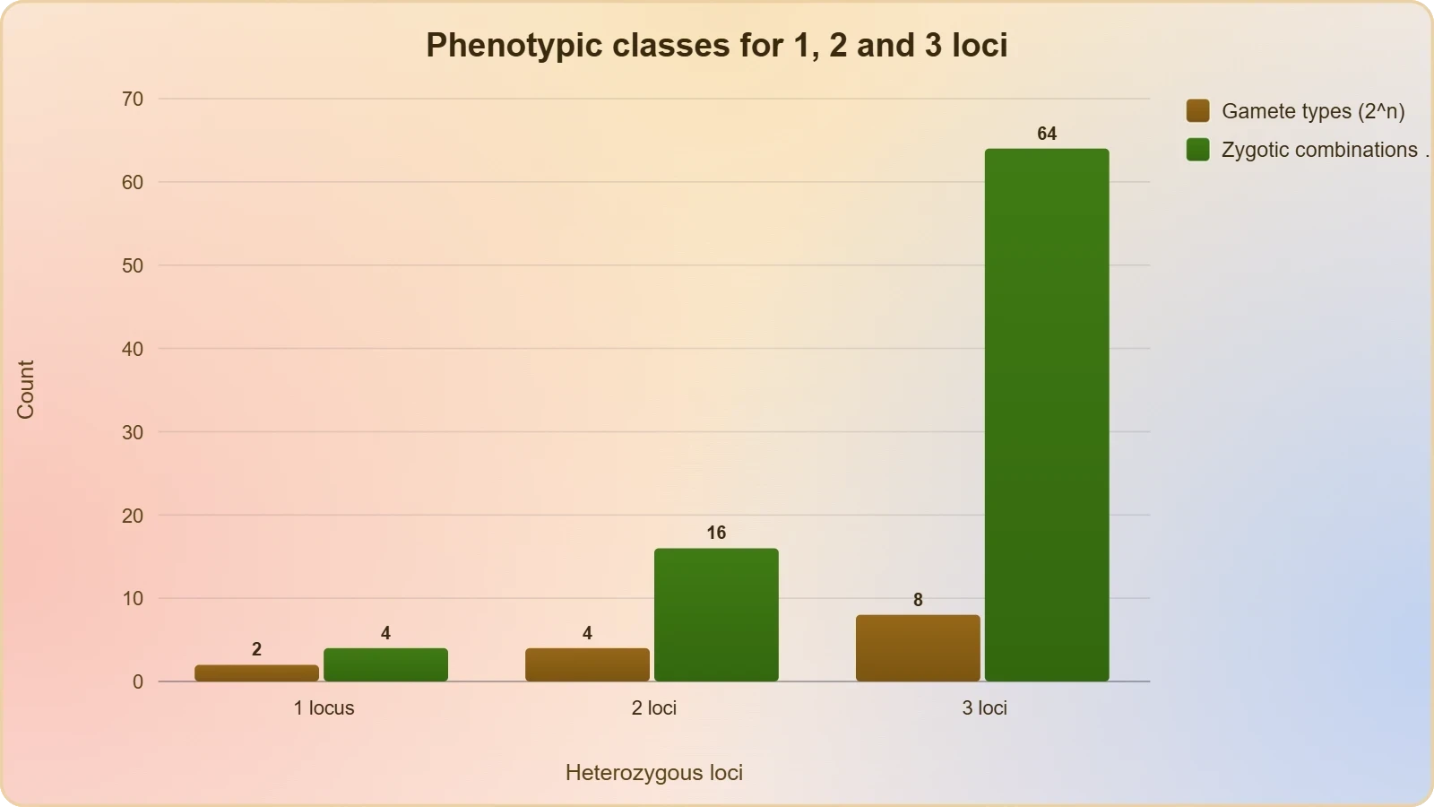
This multiplicative logic extends to any number of independently assorting loci. Three characters give a 27:9:9:9:3:3:3:1 ratio across sixty-four equally likely combinations, and n heterozygous loci give ##2^n## gamete types and ##4^n## zygotic combinations. The genotypic ratio at F2 is not 9:3:3:1; it is a longer series in which the four phenotypic classes conceal several genotypes. Round yellow seeds, for example, include RRYY, RRYy, RrYY, and RrYy, and only the last of these breeds true for neither character. Distinguishing genotype from phenotype inside each class is a routine examination skill and a frequent source of error.
Probability Tools: Product Rule and Sum Rule
Genetics is applied probability, and two rules carry most of the load. The product rule states that the probability of two independent events occurring together is the product of their separate probabilities. The sum rule states that the probability of either of two mutually exclusive events occurring is the sum of their probabilities. In a dihybrid cross the two loci are independent events, so the product rule converts any two-locus question into two one-locus questions multiplied together. This is the single most useful computational habit in the entire subject, and it scales to three or more loci without additional machinery.
Consider a cross between RrYy and RrYy and ask for the probability of a round green offspring. At the shape locus, Rr crossed with Rr gives three quarters round. At the colour locus, Yy crossed with Yy gives one quarter green. The product rule gives three sixteenths, matching the 3:16 class in the grid. Ask instead for offspring that are round green or wrinkled yellow, and the sum rule adds the two mutually exclusive probabilities, giving six sixteenths. The grid and the probability rules must always agree; when they do not, an arithmetic slip has occurred somewhere.
Worked Example: A Testcross with Two Loci
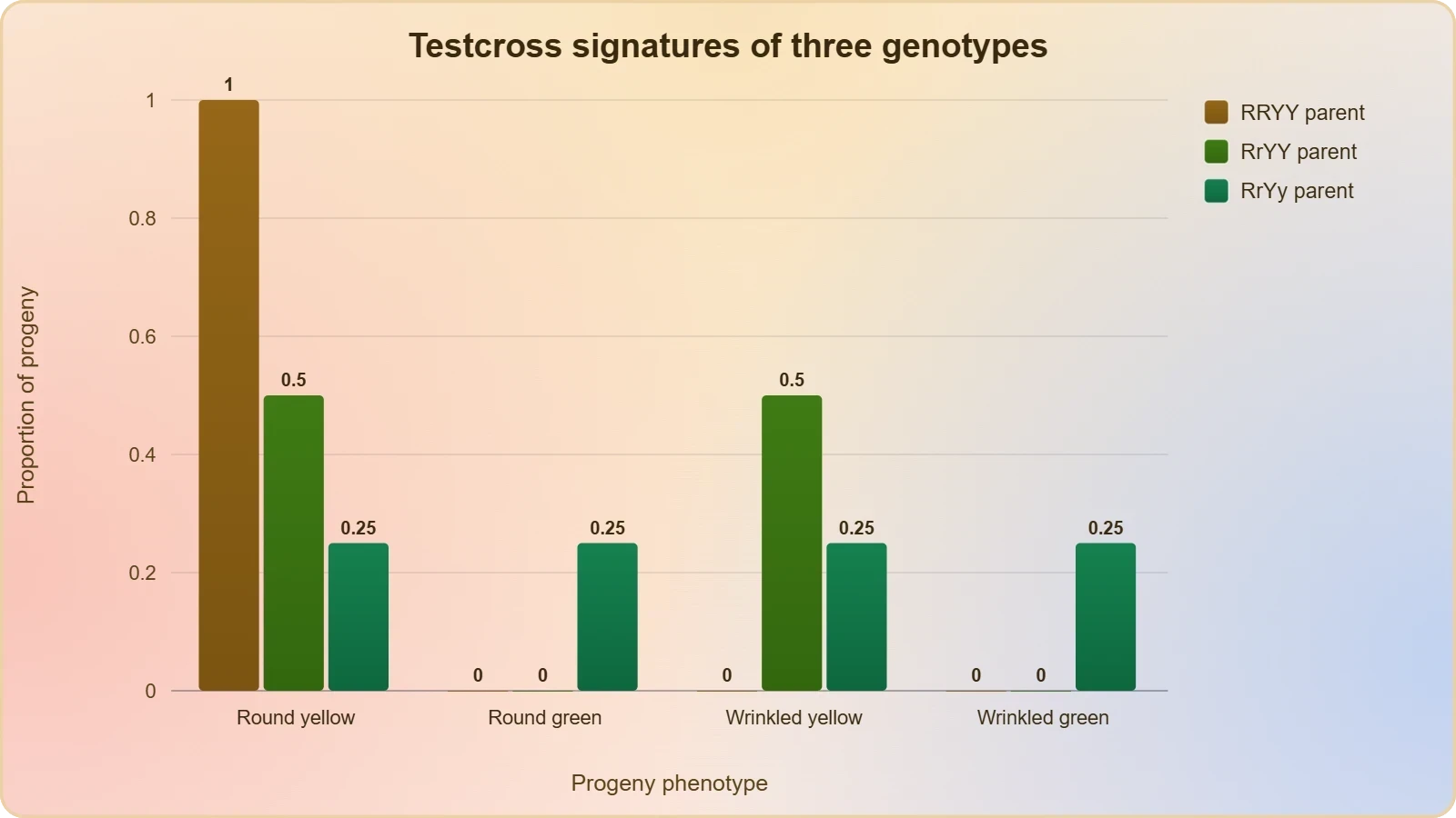
Suppose an unknown plant with round yellow seeds is crossed to a wrinkled green tester, rryy. The tester contributes only ry gametes, so the offspring phenotypes directly reveal the gametes produced by the unknown parent. If the unknown is RrYy, it produces RY, Ry, rY, and ry in equal quarters, and the progeny appear as one quarter round yellow, one quarter round green, one quarter wrinkled yellow, and one quarter wrinkled green. This 1:1:1:1 outcome is the diagnostic signature of a dihybrid heterozygote in a testcross, and it is the cleanest experimental demonstration of independent assortment available to a student.
If instead the unknown were RRYY, all progeny would be round yellow. If it were RrYY, half would be round yellow and half wrinkled yellow. Each parental genotype therefore generates a distinct progeny signature, which is why testcrosses remain a standard analytical tool. The same logic applies to three-point testcrosses used in mapping, where the rarest progeny classes reveal the double crossovers. Working through these cases by hand, predicting the ratio before drawing the square, and then verifying against the grid builds the intuition that examination questions reward.
Worked Example: Three Independently Assorting Loci
Extend the reasoning to a cross of AaBbCc with AaBbCc. The probability of offspring showing all three dominant phenotypes is the product of three independent three-quarter probabilities, which is twenty-seven sixty-fourths. The probability of all three recessive phenotypes is one sixty-fourth. The probability of exactly two dominant phenotypes requires the sum rule over three mutually exclusive arrangements, each contributing nine sixty-fourths, for a total of twenty-seven sixty-fourths. Notice that the full phenotypic series, 27:9:9:9:3:3:3:1, is simply the expansion of ##(3+1)^3##, and the general case for n heterozygous loci is ##(3+1)^n##.
This binomial structure is worth internalising because it converts apparently formidable problems into arithmetic. A question asking for the fraction of offspring homozygous at all three loci in the same cross is answered by multiplying one half by one half by one half, giving one eighth, since each locus independently yields one half homozygosity. Questions asking for a specific genotype follow the same pattern with quarters and halves substituted appropriately. The discipline of decomposing a multi-locus question into single-locus questions, applying the product rule, and then combining with the sum rule where alternatives exist, is the whole method.
Independent Assortment and the Behaviour of Chromosomes
Mendel published in 1865 and was largely ignored for thirty-five years. Communication was slow, his discrete non-blending factors seemed incompatible with the continuous variation biologists actually observed, and his use of mathematics in a biological argument struck contemporaries as foreign. Above all, he could offer no physical evidence for what his factors were made of. The rediscovery came in 1900, when de Vries, Correns, and von Tschermak independently reached his conclusions, by which time improved microscopy had revealed chromosomes that doubled and divided before each cell division. By 1902 the choreography of meiosis was mapped, and the parallel with Mendelian segregation became impossible to ignore.
Walter Sutton and Theodor Boveri noticed that chromosomes and genes behave alike in three respects: both occur in pairs, both segregate at gamete formation so that only one of each pair enters a gamete, and independent pairs segregate independently of one another. Sutton united chromosomal behaviour with Mendelian principles under the name chromosomal theory of inheritance. The cytological basis of independent assortment is visible during anaphase of meiosis I, when two chromosome pairs align at the metaphase plate independently. One long orange chromosome may travel with a short green partner, or with a short red partner, with equal likelihood.
Why Independent Assortment Requires Separate Chromosomes
The law holds cleanly only when the two gene pairs lie on different chromosomes, or far enough apart on the same chromosome that crossing over separates them freely. Genes on separate chromosomes are physically unconnected during meiosis, so their alignment orientations are independent, and the four gamete types appear in equal quarters. Genes on the same chromosome are another matter entirely. They tend to travel together, and the parental combinations appear in excess of the recombinant ones. This is the modification that Morgan's work forced upon Mendel's second law, and it is the bridge to the next lesson on linkage.
Even within a single chromosome, distance matters. Two loci near opposite ends of a long chromosome behave almost as if they were on separate chromosomes, because at least one crossover between them is nearly certain. Two loci close together are rarely separated and behave as a linked unit. The practical rule is that independent assortment is the default for unlinked loci and an approximation for distant linked loci, with the approximation improving as recombination frequency approaches fifty per cent. Fifty per cent recombination is the ceiling, because even perfect linkage cannot produce more recombinant gametes than the independent case.
Recombination Frequency as a Measure of Independence
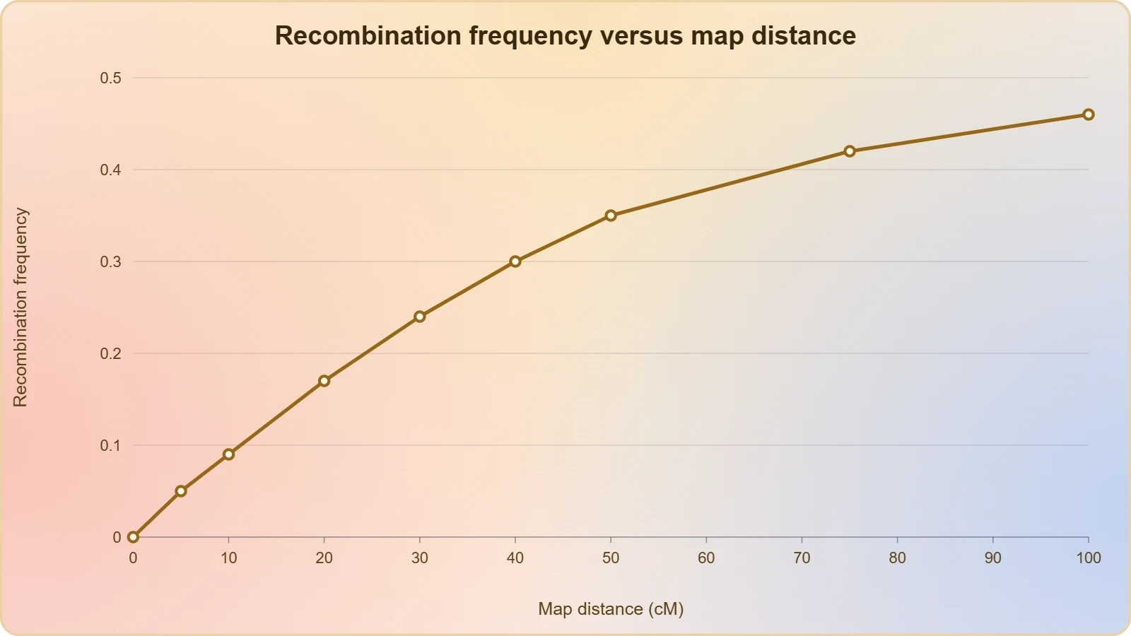
Recombination frequency is defined as the proportion of offspring showing non-parental combinations of alleles, and it quantifies how far independent assortment has been achieved. A value of fifty per cent means the loci assort independently; a value near zero means they are tightly linked. Morgan found that white and yellow in Drosophila recombined at only 1.3 per cent, while white and miniature wing recombined at 37.2 per cent, demonstrating that linkage strength varies continuously. Alfred Sturtevant, Morgan's student, recognised that recombination frequency could serve as a map distance, and one per cent recombination was defined as one map unit, or centimorgan.
This insight converted genetics from a descriptive discipline into a cartographic one. By compiling recombination frequencies among many gene pairs, Sturtevant produced the first genetic maps of Drosophila chromosomes, ordering loci linearly and spacing them according to recombination. The mathematics is straightforward: for two loci with recombination frequency ##r##, the four gamete classes are not equal quarters but ##(1-r)/2## for each parental type and ##r/2## for each recombinant type. Setting ##r = 0.5## recovers the independent case of one quarter each, which shows that independent assortment is simply the limiting case of linkage at maximum distance.
Linkage, Recombination, and the Limits of Mendel's Second Law
Morgan's dihybrid crosses in Drosophila were designed exactly like Mendel's pea crosses, but the results refused to cooperate. Crossing yellow-bodied, white-eyed females with brown-bodied, red-eyed males and intercrossing the F1 progeny produced an F2 ratio that deviated sharply from 9:3:3:1. The parental combinations were far too common and the recombinant combinations far too rare. Morgan knew the genes in question sat on the X chromosome, and he concluded that genes physically associated on a chromosome tend to be inherited together. He named this association linkage and named the generation of non-parental combinations recombination.
Linkage is not an all-or-nothing phenomenon. Morgan's group found tightly linked genes with very low recombination and loosely linked genes with higher recombination, and the white-yellow and white-miniature comparisons quantified the difference. The mechanism is crossing over during prophase of meiosis I, when homologous chromosomes exchange segments. A crossover between two loci separates the alleles that were travelling together; a crossover elsewhere on the chromosome does not. The probability of a separating crossover therefore rises with the distance between loci, which is why recombination frequency is a usable proxy for map distance.
How Linkage Modifies the 9:3:3:1 Expectation
When two loci are linked, the F1 heterozygote does not produce four gamete types in equal quarters. If the parental chromosomes carried R with Y and r with y, the parental gametes RY and ry are over-represented and the recombinants Ry and rY are under-represented. The F2 phenotypic ratio then shifts away from 9:3:3:1, typically inflating the parental phenotypic classes and shrinking the recombinant ones. The deviation is diagnostic: a ratio close to 9:3:3:1 indicates independent assortment, while a significant excess of parental classes indicates linkage. The magnitude of the deviation measures the recombination frequency.

This is the precise sense in which Mendel's second law was modified rather than overturned. The law remains correct for genes on different chromosomes and for genes sufficiently far apart on the same chromosome. It fails only for linked genes, and even then the failure is quantitative rather than absolute. Modern genetics therefore treats independent assortment as the baseline expectation and linkage as the informative exception, which is exactly why recombination data are so valuable for mapping. The next lesson develops the chromosomal theory and linkage in full cytological detail.
Common Errors and How to Avoid Them
The most frequent mistake is assuming that a 9:3:3:1 ratio implies a 9:3:3:1 genotypic ratio. It does not; nine genotypes underlie the four phenotypes, and only rryy is fully homozygous recessive. A second error is writing gametes without ensuring that each carries exactly one allele from each locus, producing invalid types such as RR or Yy. A third is confusing the product and sum rules, adding probabilities that should be multiplied or multiplying those that should be added. A fourth is forgetting that independent assortment requires unlinked loci, then applying 9:3:3:1 to a cross that plainly shows linkage.
Another trap is misreading dominance when a dihybrid cross involves a locus with incomplete dominance, which changes the expected ratio from 9:3:3:1 to 3:6:3:1:2:1 across six phenotypic classes. Similarly, epistasis, in which one locus masks another, produces characteristic distortions such as 9:7 or 12:3:1. Recognising these modified ratios as signatures of specific interactions is a higher-order skill that distinguishes a competent student from an excellent one. Always check whether the assumptions behind 9:3:3:1 actually hold before invoking it.
Genetic Diversity and the Wider Significance of Assortment
Independent assortment is one of the principal engines of genetic diversity in sexually reproducing organisms. With two heterozygous loci, four gamete types arise; with three, eight; with n, ##2^n##. In humans, twenty-three chromosome pairs can be arranged at metaphase I in ##2^{23}##, roughly 8.4 million, different combinations, before crossing over is even considered. Crossing over multiplies this further, so that a single human couple can in principle produce a staggeringly diverse array of offspring. This combinatorial richness is the raw material on which natural selection acts, and it explains why sexual reproduction persists despite its considerable costs.
The agricultural and medical implications are direct. Plant breeders exploit independent assortment when combining desirable traits from different varieties, predicting the frequencies of superior genotypes in segregating generations. In human genetics, the same logic underlies risk calculations for offspring of parents carrying different recessive conditions. The 9:3:3:1 ratio and its probability machinery are not examination ornaments; they are the working tools of anyone predicting inheritance outcomes, from a wheat breeder selecting for rust resistance and yield to a counsellor estimating the chance of a child inheriting two independent disorders.
From Mendel's Factors to the Modern Synthesis
Mendel's factors became genes, genes became DNA sequences, and independent assortment became a statement about the behaviour of chromosomes at meiosis. The conceptual continuity is remarkable: the same 9:3:3:1 ratio that emerged from counting pea seeds in a monastery garden reappears in genome-wide association studies as the expected distribution of unlinked markers. What changed is the resolution of the explanation, not the logic of the prediction. The law survived because it captured something real about the physical independence of chromosomes, and it was refined rather than replaced when linkage revealed its boundaries.
Modern genomics has added nuance without disturbing the core. Genes on different chromosomes assort independently, genes far apart on the same chromosome approximate independence, and genes close together are linked. Whole-genome sequencing now allows recombination frequencies to be measured directly in pedigrees and populations, confirming the map distances Sturtevant inferred from visible markers a century ago. The dihybrid cross, in this light, is not a historical curiosity but the simplest experimental window onto a principle that operates across every sexually reproducing species on the planet.
Consolidating the Lesson
The dihybrid cross follows two characters at once and yields the 9:3:3:1 phenotypic ratio when the loci assort independently. That ratio is the product of two 3:1 monohybrid ratios, and it can be derived by Punnett square, by binomial expansion, or by the product and sum rules of probability. Independent assortment reflects the independent orientation of chromosome pairs at metaphase I, and it holds for genes on separate chromosomes or far apart on the same one. Linkage, discovered by Morgan in Drosophila, is the exception that refines the law, quantified by recombination frequency and exploited by Sturtevant for genetic mapping.
Before moving to the chromosomal theory and linkage, verify that you can construct a sixteen-cell Punnett square from gamete enumeration, derive the 9:3:3:1 ratio algebraically, apply the product and sum rules to unfamiliar questions, and explain why linked genes deviate from the Mendelian expectation. These four competencies form the foundation for everything that follows, from three-point mapping to the analysis of polygenic traits and human genetic disorders. The next lesson takes the chromosomal theory of inheritance and the mechanics of linkage as its subject, building directly on the cytological foundations established here.
Also Read
- No links available.
From our network :
- Analyzing Trump Deportation Numbers Insights Into The 2026 Immigration Crackdown
- How to Print Cheaply: Cutting the Cost per PageA practical, measured guide to lowering what each printed page costs — duplex and draft modes, third-party ink, yield mathematics, and knowing when a new printer beats refills.
- Where to Put Your Wireless Router for Better CoverageA practical, physics-grounded guide to router placement: why the centre of the home beats the corner, how walls and metal sap signal, and how to run a simple survey that proves the improvement.
- EV 2.0: The Solid-State Battery Breakthrough and Global Factory ExpansionDiscover the impact of the Solid-State Battery Breakthrough on the EV market. Learn about CATL and BYD stock growth, global factory expansion in Europe, and the future of EV 2.0 technology.
- Do You Need a New Router or Is Your Internet Plan the Problem?A practical comparison of the signs that point to router limits versus signs your broadband speed or provider is the bottleneck, so you can decide what to replace before spending money.
- 98% of Global MBA Programs Now Prefer GRE Over GMAT Focus EditionExplore why 98% of global MBA programs now prefer the GRE over GMAT Focus. Learn about the shorter GRE format, verbal logic importance, and strategic versatility for students.
- 10 Physics Numerical Problems with Solutions for IIT JEEPrepare for IIT JEE with 10 physics numerical problems, complete with detailed solutions and conceptual explanations. Ideal for mastering kinematics, thermodynamics, electromagnetism, and optics.
- AI-Powered 'Precision Diagnostic' Replaces Standard GRE Score ReportsDiscover the new GRE Precision Diagnostic. Learn how AI-powered behavioral analytics and time-to-solve tracking are replacing standard GRE score reports to empower students.
- Trump Political Strategy How Geopolitical Stunts Serve As Media Diversions
RESOURCES
- 4.2.2: Dihybrid Crosses and Independent Assortmentbio.libretexts.orgThe dihybrid crosses that Mendel performed consistently revealed the 9:3:3:1 ratio in dihybrid crosses, leading him to conclude that the factors controlling the ...
- 2.4 A Dihybrid Cross Showing Mendel's Second Law (Independent ...opengenetics.pressbooks.tru.ca2.4 A Dihybrid Cross Showing Mendel's Second Law (Independent Assortment) ... Mendel found that each locus had two alleles that segregated themselves during the ...
- 12.3: Dihybrid Crosses and Mendel's Law of Independent Assortmentbio.libretexts.orgDec 16, 2021 ... The law of independent assortment states that a gamete into which an r allele sorted would be equally likely to…
- Learn and try: The law of independent assortment - Khan Academykhanacademy.orgIf the seed color and seed shape genes were in fact always inherited as a unit, or completely linked, a dihybrid cross should produce…
- dihybrid cross / dihybrid | Learn Science at Scitable - Naturenature.comIn 1865, Gregor Mendel performed dihybrid crosses on pea plants and discovered a fundamental law of genetics called the Law of Independent Assortment.
- Law of Independent Assortment - BYJU'Sbyjus.comMendel's Experiment on the Law of Independent Assortment ... The Law of Independent Assortment states that during a dihybrid cross (crossing of two pairs…
- Dihybrid Cross Question W Answer Key Complete Guidewww2.american-usa.comTypically, these traits follow Mendel's laws of inheritance, particularly the Law of Independent Assortment, which states that the alleles of two (or more) ...
- 12.3 Laws of Inheritance - Biology 2e | OpenStaxopenstax.orgMar 28, 2018 ... The independent assortment of genes can be illustrated by the dihybrid cross, a cross between two true-breeding parents that express ...
- Laws of Inheritance - OERTXoertx.highered.texas.govThe independent assortment of genes can be illustrated by the dihybrid cross, a cross between two true-breeding parents that express different traits for ...
- Law of Independent Assortment — Definition & Role - Expiiexpii.comGenes and Math: Dihybrid Crosses and Offspring Ratios. In Mendel's dihybrid cross experiments, heterozygous parents always produced the same ratio of offspring ...
- Unlocking the Secrets of Heredity: How Dihybrid Inheritance ...ftp.acp-mn.com7 days ago ... Building upon the foundational work of Gregor Mendel, dihybrid crosses illustrate the independent assortment of genes, a cornerstone of modern ...
- Clarifying Mendelian vs non-Mendelian inheritance - PMC - NIHpmc.ncbi.nlm.nih.govMay 28, 2024 ... b) According to Mendel's law of independent assortment, when 2 genes ... dihybrid crosses (Fig. 1b). Deviations from this 9:3:3:1…
- Dihybrid Inheritance & Independent Assortment | PDF - Scribdscribd.comThis document discusses Mendel's dihybrid cross experiments and the law of independent assortment. [1] It compares monohybrid and dihybrid crosses, noting ...
- MENDELIAN DIHYBRID CROSS What phenotypic ratio is obtained ...facebook.comOct 13, 2026 ... ... dihybrid cross demonstrates Mendel's Law of Independent Assortment, assuming the genes assort independently. Can you recall all four ...
- Dihybrid Cross Definition and Example - Genetics - ThoughtCothoughtco.comMay 12, 2025 ... Dihybrid cross-pollination experiments led Gregor Mendel to develop his law of independent assortment. This law states that alleles are ...