The Race to See the Invisible: How Fast Biosensors Could Transform Nanoplastic Monitoring

Nanoplastics are the invisible endgame of plastic pollution: particles so small that ordinary filtration, microscopy, and routine field sampling can miss them entirely. A newly reported biosensor promises to identify these particles in water within minutes, attacking one of environmental science’s most stubborn bottlenecks—the gap between contamination and trustworthy measurement. The breakthrough matters because pollution that cannot be measured cannot be managed intelligently.

The central story is not merely that a sensor is fast. It is that rapid detection could redesign the entire monitoring workflow, moving analysis from distant laboratories toward treatment plants, rivers, reservoirs, coastlines, and industrial sites. Nanoplastics behave differently from larger fragments, interact strongly with biological surfaces, and often exist alongside salts, organic matter, microbes, and other microscopic debris.

This analysis explains why nanoplastics are technically difficult to detect, how biosensing principles convert molecular recognition into a measurable signal, what a minute-scale readout can and cannot prove, and why speed must be matched by calibration, selectivity, and transparent validation. The decisive question is not whether a device produces a quick signal, but whether that signal reliably represents nanoplastic contamination in real water.

The Nanoplastic Problem Begins with Scale

Plastic pollution is often pictured as bottles, bags, fibres, and fragments that can be collected or counted. Nanoplastics overturn that comfortable picture. They are generally discussed as plastic particles in the nanoscale regime, although a universally enforced lower and upper boundary remains difficult because definitions vary across research communities. Their small size creates enormous surface area relative to mass and gives them unusual transport, aggregation, and biological-interaction behaviour.

Detection is therefore a problem of both physics and chemistry. A water sample may contain particles with different polymers, shapes, weathering histories, surface charges, and attached contaminants. The analyst must distinguish those particles from mineral colloids, dissolved organic matter, lipids, cell debris, and microbial structures. A rapid biosensor is valuable precisely because it can introduce selective molecular recognition into a sample that conventional size-based inspection cannot interpret alone.

Why Nanoplastics Evade Routine Observation

At larger dimensions, researchers can combine filtration, spectroscopy, microscopy, and visual classification to establish that a fragment is plastic. At nanoscale dimensions, the signal from an individual particle becomes weak, while the surrounding water matrix becomes comparatively influential. Light scattering, for example, depends strongly on particle size, refractive index, wavelength, and aggregation state. A tiny polymer particle may be physically present yet produce no convenient visual signature.

The problem intensifies because nanoplastics are not a single chemically uniform substance. Polyethylene, polypropylene, polystyrene, polyethylene terephthalate, and other polymers differ in density, aromaticity, oxidation behaviour, and surface chemistry. Sunlight, mechanical abrasion, heat, and microbial activity can introduce oxygen-containing groups or alter roughness. Consequently, a sensor designed around one pristine laboratory particle may behave differently when confronted with weathered material from a river or wastewater stream.

Size also changes transport. Small particles can remain suspended, pass through conventional barriers, associate with colloids, or move through porous media in ways that larger fragments cannot. Their behaviour depends on ionic strength, pH, dissolved organic carbon, and interactions with minerals and biological macromolecules. The important conclusion is blunt: “plastic present” is not a complete analytical description. A meaningful result must identify what kind of particle was detected, in what concentration, and under which water conditions.

The Measurement Bottleneck in Environmental Surveillance

Traditional workflows often require several stages: collecting a representative volume, removing interfering material, concentrating particles, separating fractions, identifying polymer chemistry, and quantifying the result. Each stage can introduce loss or contamination. Plastic laboratory equipment, airborne fibres, sample containers, and filtration membranes can all complicate blank correction. The final answer may arrive after the environmental conditions have already changed.

Suppose a monitoring team samples a treatment outlet after rainfall. If preparation and instrumental analysis take days, the team may discover elevated contamination only after the discharge event has passed. A fast screen changes the operational question from “What was present last week?” to “Should we investigate this water now?” That does not make the sensor a complete replacement for high-resolution analysis; it makes it a powerful triage instrument.

The value of speed can be described through a simple monitoring model. If a workflow processes one sample every ##[t##sub##analysis##]## minutes, then its nominal hourly capacity is ##[R = \dfrac{60}{t##sub##analysis##}]## samples per hour. Reducing analysis time from 120 minutes to 10 minutes raises nominal capacity from 0.5 to 6 samples per hour, before accounting for sampling, cleaning, and quality-control overhead.

This first calculation is not a claim about the reported biosensor’s exact throughput. It is a derivation of why minute-scale analysis matters operationally. Real systems must include calibration, sample handling, duplicate measurements, and instrument recovery. Even so, the arithmetic exposes the strategic advantage: rapid detection allows denser spatial sampling, faster source tracing, and more immediate decisions about additional laboratory confirmation.

How a Biosensor Turns Recognition into a Readout

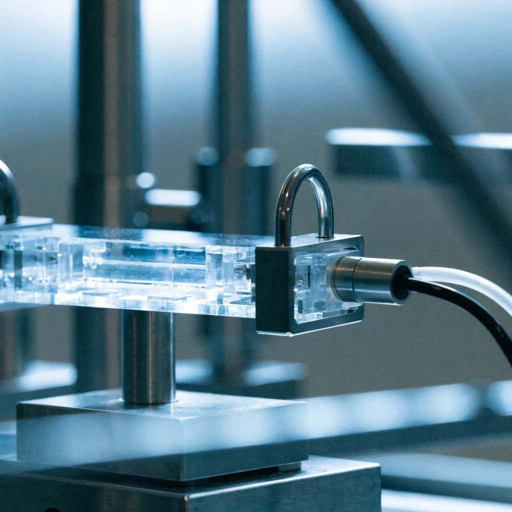
A biosensor combines a recognition element with a transducer. The recognition element may interact with a polymer surface, a coating, an engineered ligand, an antibody-like binding structure, a nucleic-acid-based element, or another selective interface. The transducer converts binding or particle capture into an optical, electrical, electrochemical, mechanical, or thermal response. The instrument then maps that response to a calibrated estimate or screening threshold.

The elegance of the approach lies in its division of labour. Chemistry supplies selectivity; physics supplies measurability; electronics and software supply speed. Yet the device is not “seeing plastic” in the ordinary sense. It is detecting a target-associated change in a measurement channel. That distinction matters because every biosensor has a recognition envelope, a dynamic range, a detection limit, and a susceptibility to matrix effects.

Recognition, Binding, and Selectivity

Selective capture is the heart of the technology. If the sensor surface binds preferentially to a nanoplastic-associated feature, particles accumulate where the transducer can detect them. That feature may be a polymer-specific surface chemistry, a common plastic additive, a weathering product, or a deliberately introduced assay label. The stronger and more selective the interaction, the easier it becomes to distinguish the target from background material.

Binding is rarely an all-or-nothing event. A simple equilibrium description uses an association constant, written inline as ##[K##sub##a##]##, and a dissociation constant, ##[K##sub##d##]##. For a target concentration ##[C]##, an idealized fractional occupancy can be represented as ##[\theta=\dfrac{C}{K##sub##d##+C}]##. This model is simplified, but it clarifies why signal rises rapidly at low concentrations and eventually approaches saturation.

The second calculation shows that when target concentration equals the dissociation constant, half of the idealized binding capacity is occupied. A low ##[K##sub##d##]## indicates stronger apparent binding, but strength alone is not enough. Excessively sticky surfaces may capture unrelated colloids, become difficult to regenerate, or saturate before the sample can be quantified. High-quality design balances affinity, selectivity, reversibility, and performance in authentic water.

Transduction: Optical, Electrical, and Mechanical Signals

Once recognition occurs, the sensor must translate it into a signal. Optical systems may measure changes in colour, fluorescence, absorbance, scattering, or resonance. Electrical systems may monitor impedance, capacitance, current, or potential. Mechanical systems can detect mass loading or changes in resonant frequency. The best format is not necessarily the most sophisticated one; it is the format that preserves useful selectivity under field conditions.

Signal-to-noise ratio is a decisive engineering criterion. If the measured signal is ##[S]## and the standard deviation of background noise is ##[\sigma##sub##b##]##, a basic screening ratio is ##[\mathrm{SNR}=\dfrac{S}{\sigma_b}]##. A sensor can be fast yet useless if its background varies as much as its target response. Conversely, a modest signal may be entirely practical when the baseline is stable and the calibration is well controlled.

The third calculation gives an illustrative signal-to-noise ratio of six. It does not establish a regulatory detection limit, because that requires replicated blanks, low-level standards, matrix-matched samples, and a defined decision rule. Still, it demonstrates the logic behind rapid readouts: the device must produce a signal that is not merely large, but reliably separated from the variability of clean and contaminated water backgrounds.

What “Within Minutes” Changes in the Field

A minute-scale biosensor can compress the distance between observation and intervention. Inspectors could screen multiple locations along a river, compare influent and effluent, test water before and after filtration, or identify unusual spikes around industrial activity. Water utilities could use rapid measurements to decide when to trigger a more exhaustive analytical protocol. Researchers could generate denser time-series data instead of relying on occasional samples.

That speed has a second consequence: it changes sampling strategy. Slow, expensive methods encourage sparse sampling and carefully selected sites. Faster tools permit adaptive sampling, in which an initial result determines where the next sample is collected. This is especially important for pollutants that are patchy, episodic, or strongly affected by flow, rainfall, tidal movement, and treatment conditions.

From Occasional Laboratory Tests to Adaptive Monitoring

Environmental contamination is rarely uniform. A single bottle of water may not represent a whole reservoir, discharge channel, or groundwater plume. Rapid screening allows investigators to increase replication and map gradients. A high reading can be followed upstream; a low reading can prevent unnecessary deployment of expensive analytical equipment. The sensor becomes a decision instrument, not merely a smaller version of a laboratory machine.

Consider a simple uncertainty model for an average concentration. If independent measurements have standard deviation ##[\sigma]## and the team collects ##[n]## replicates, the standard error of the mean is ##[\mathrm{SE}=\dfrac{\sigma}{\sqrt{n}}]##. Increasing replicates from 4 to 25 reduces the multiplier from 0.5 to 0.2. Faster assays make that statistical improvement more affordable because each additional observation consumes less time.

The fourth calculation illustrates a practical gain in precision: five replicates produce a standard error of 2 units under the stated assumptions, compared with 5 units for four replicates. The example assumes independent observations and stable variance, conditions that field data may violate. Even with those limitations, the principle is decisive: rapid detection can improve confidence not by mathematical magic, but by making better sampling economically realistic.

Screening Is Not the Same as Definitive Identification

Speed must not be confused with certainty. A biosensor may indicate the presence of a nanoplastic-related target, estimate a concentration range, or flag a sample for confirmation. It may not identify every polymer type, particle shape, additive, weathering state, or biological hazard. Confirmatory methods such as spectroscopy, chromatography, mass spectrometry, electron microscopy, or orthogonal particle analysis may still be necessary.

Detection limits require disciplined definition. One common conceptual form is ##[\mathrm{LOD}=\mu_{\mathrm{blank}}+k\sigma_{\mathrm{blank}}]##, where the multiplier ##[k]## depends on the chosen statistical and regulatory framework. The limit is therefore not an eternal property of the sensor alone. It depends on sample matrix, preparation, calibration model, replicate number, blank contamination, and the acceptable balance between false positives and false negatives.

The fifth and final calculation produces an illustrative detection threshold of 0.35 signal units. It is deliberately framed as an example rather than a performance claim. A credible nanoplastics detection platform must report how that threshold was obtained, how many blanks were measured, which water matrices were tested, and whether independent methods confirmed the result. Without that evidence, “within minutes” describes speed, not analytical validity.

The Scientific Standard for Trustworthy Nanoplastic Detection

The reported advance deserves attention because measurement is the foundation of environmental policy. However, enthusiasm should be paired with rigorous questions. What particle sizes can the sensor detect? Does it distinguish polymer classes? How does dissolved organic matter affect the response? Can the device tolerate turbidity and salinity? Does it measure particle number, mass, surface area, or an indirect proxy? These details determine whether the innovation is transformative or merely convenient.

Validation must occur across realistic conditions rather than only clean water spiked with uniform laboratory spheres. Authentic samples contain mixtures, weathered particles, biofilms, mineral coatings, and unknown interferents. The most persuasive evidence will compare rapid biosensor readings with established reference methods across wastewater, freshwater, drinking-water sources, coastal water, and industrial discharge. Reproducibility between operators and instruments will matter as much as headline response time.

Calibration, Matrix Effects, and Quality Control

Calibration converts a physical response into an estimate. That conversion can be linear over a narrow range, nonlinear near saturation, or distorted by aggregation and competitive binding. Matrix effects arise when salts, pH, dissolved carbon, surfactants, suspended solids, or microbial products alter recognition or transduction. Therefore, a calibration curve prepared in ultrapure water may fail when transferred directly to a river or treatment plant.

Quality control should include procedural blanks, field blanks, negative controls, positive controls, spike recovery, replicate measurements, and, where feasible, independent confirmation. Recovery experiments reveal whether sample preparation loses particles. Blanks reveal contamination from tubing, containers, air, or consumables. Controls reveal whether the recognition chemistry is responding to the intended target rather than a generic increase in particulate material.

Portable deployment also introduces human factors. A field device needs simple sample handling, stable reagents, clear error messages, battery resilience, contamination-resistant components, and a result that communicates uncertainty rather than presenting false precision. Data should carry metadata such as time, location, temperature, pH, conductivity, turbidity, and sample volume. Without that context, a rapid number can be difficult to compare across sites or seasons.

Health Relevance and the Limits of the Current Evidence

Nanoplastics attract concern because their dimensions may permit interactions with cells, proteins, membranes, and biological barriers that differ from those of larger particles. They may also carry additives or adsorbed chemicals. Yet exposure risk cannot be inferred from detection alone. Toxicological significance depends on dose, size distribution, polymer composition, shape, surface chemistry, residence time, route of exposure, and the biological system under study.

A fast environmental sensor should therefore be understood as an exposure-information tool, not a complete health-risk calculator. Its contribution is to reveal where particles occur, how concentrations vary, and which water systems require deeper investigation. That information can strengthen toxicology, epidemiology, and treatment research. It can also prevent resources from being wasted on vague claims unsupported by reliable measurements.

The strongest future systems will combine rapid biosensing with orthogonal confirmation and open reporting. They will distinguish screening signals from validated concentrations, state uncertainty honestly, and publish performance across real matrices. In that framework, the biosensor’s greatest achievement is not replacing every laboratory instrument. It is making nanoplastic surveillance frequent, spatially resolved, and responsive enough to guide action before contamination becomes an entrenched environmental record.