
Geometric abstract lines and intersections
The mathematical analysis of linear systems of equations lies at the absolute core of classical algebra, functional analysis, and modern computational science. When modeling real-world physical systems, engineering structures, or optimization networks, researchers inevitably encounter systems of algebraic relations. These systems govern how vectors transform, how physical forces equilibrate, and how constraints intersect within high-dimensional Euclidean spaces. The behavior of these systems—whether they possess a singular, unique equilibrium, an infinite spectrum of configurations, or no possible physical solution—can be systematically classified through both graphical and rigorous algebraic methods.
From a spatial and geometric perspective, linear equations define affine manifolds such as lines, planes, or hyperplanes within a vector space. The solution to a system of equations corresponds precisely to the intersection of these manifolds. When these geometric entities align or run parallel to one another, the system transitions from a determined state to a singular or rank-deficient state. Analyzing these transitions requires a deep synthesis of Euclidean geometry, linear dependency, matrix theory, and the algebraic principles that dictate consistency and inconsistency in vector spaces.
This academic inquiry explores the deep theoretical mechanics governing the solubility of linear systems. By examining the geometric behaviors of lines and planes alongside advanced algebraic framework configurations, we establish a robust paradigm for understanding systems with infinite solutions and those with no solutions. Through a series of fifteen structured mathematical problems, rigorous derivations, and thematic comparative datasets, we will dissect the concepts of matrix singularity, rank classifications, numerical stability, and real-world computational mechanics.
On This Page
- Geometric abstract lines and intersections
- 1. The Geometric Underpinnings of Linear Systems: Dimensionality and Trajectories
- 2. Algebraic Analysis of Inconsistency and Linear Dependency
- 3. Advanced Mathematical Derivations and Parameterizations
- 4. Computational Strategies and Numerical Stability in Real-World Systems
- 5. Physical and Engineering Applications of Linear Systems
1. The Geometric Underpinnings of Linear Systems: Dimensionality and Trajectories
To grasp the behavior of a system of equations, we must first map its algebraic statements onto a geometric canvas. Within the context of a two-dimensional Euclidean space, denoted as ##[\mathbb{R}^2]##, a single linear equation of the form ##[ax + by = c]## represents a one-dimensional manifold, or line. This line represents the continuous locus of all coordinate pairs ##[(x, y)]## that satisfy the linear constraint. When multiple equations are introduced, they represent multiple spatial constraints, and the solution to the system is geometrically defined as the intersection of these lines. The fundamental properties of these intersections—whether they meet at a single coordinate, merge into a single entity, or never cross—define the fundamental nature of the system's solution space.
As we extend our analysis to higher-dimensional spaces, such as ##[\mathbb{R}^3]## or ##[\mathbb{R}^n]##, these lines transition into planes and hyperplanes. In three dimensions, a linear equation describes a two-dimensional flat surface. The intersection of two planes typically yields a line, representing a system with infinitely many solutions parameterized by a single variable, while the intersection of three planes may yield a unique point. However, when these planes are parallel, or when their intersection lines do not coincide, the system lacks any mutual point of contact. This spatial perspective allows us to visually classify systems as consistent (having one or more solutions) or inconsistent (having no solutions), providing an intuitive foundation for the algebraic proofs that follow.
1.1 Collinearity, Coincidence, and Infinite Solution Spaces
Collinearity and coincidence represent the geometric state where all equations within a system describe the exact same physical line or hyperplane. In this scenario, the constraints placed upon the variables are redundant, meaning one equation can be algebraically transformed into the other via scalar multiplication. Consequently, the individual lines lie directly on top of one another, resulting in an infinite number of intersecting points. The system is described as consistent and dependent, meaning that the choice of one variable directly dictates the values of the remaining variables along the shared trajectory.
To analyze this mathematically, consider a standard system of two equations. We formulate our first mathematical problem to demonstrate how coincidence arises when the coefficients and constants scale proportionally.
Problem 1: Algebraic Condition for Coincident Lines
Let a system of two linear equations be represented generally by:
###\begin{cases} a_1 x + b_1 y = c_1 \\ a_2 x + b_2 y = c_2 \end{cases}###
Show that the lines are coincident (and thus possess infinitely many solutions) if and only if there exists a non-zero scalar ##[k \in \mathbb{R}]## such that:
###a_2 = k a_1, \quad b_2 = k b_1, \quad c_2 = k c_1###
Derivation: If the lines are coincident, they must share the same slope and y-intercept. Let us express both equations in slope-intercept form, assuming ##[b_1 \neq 0]## and ##[b_2 \neq 0]##:
###y = -\dfrac{a_1}{b_1}x + \dfrac{c_1}{b_1} \quad \text{and} \quad y = -\dfrac{a_2}{b_2}x + \dfrac{c_2}{b_2}###
For these equations to represent the identical line, their slopes must be equal:
###-\dfrac{a_1}{b_1} = -\dfrac{a_2}{b_2} \implies \dfrac{a_1}{a_2} = \dfrac{b_1}{b_2} = \dfrac{1}{k}###
This implies ##[a_2 = k a_1]## and ##[b_2 = k b_1]##. Furthermore, their y-intercepts must also be identical:
###\dfrac{c_1}{b_1} = \dfrac{c_2}{b_2} \implies c_2 = \left(\dfrac{b_2}{b_1}\right) c_1 = k c_1###
Thus, we have successfully derived the proportional scaling condition for infinite solutions: ##[\dfrac{a_1}{a_2} = \dfrac{b_1}{b_2} = \dfrac{c_1}{c_2}]##, proving the theorem.
Geometric Analysis
Linear System Geometric Classifications
A comprehensive taxonomy of linear systems based on spatial configuration and analytical consistency.
Classification of Linear Systems
A quick reference guide for determining the nature of solutions in a system of two linear equations.
| Geometric State | Algebraic Classification | Solution Count | Proportionality Condition |
|---|---|---|---|
| Intersecting | Consistent & Independent | Unique (1) | a1/a2 ≠ b1/b2 |
| Coincident | Consistent & Dependent | Infinitely Many (∞) | a1/a2 = b1/b2 = c1/c2 |
| Parallel | Inconsistent | None (0) | a1/a2 = b1/b2 ≠ c1/c2 |
- The variables a, b, and c represent coefficients of the equations ax + by = c.
- Consistent systems have at least one solution, while inconsistent systems have none.
Note:
Assumes that coefficient denominators are non-zero.
For higher-dimensional systems, the condition generalizes via rank equivalence.
1.2 Parallelism and the Inconsistency of Non-Intersecting Trajectories
Parallelism represents the geometric state where lines or hyperplanes have identical orientation vectors but are separated by a constant spatial distance. In ##\mathbb{R}^2##, two parallel lines share the same slope but possess distinct y-intercepts. Because they are parallel, they never intersect, regardless of how far they are extended. Consequently, there is no coordinate pair ##[(x, y)]## that can satisfy both linear constraints simultaneously. The system is classified as inconsistent, reflecting a logical contradiction where the equations demand conflicting properties of the underlying variables.
To mathematically characterize parallel systems, we analyze the relationship between their coefficients and constant terms. Let us formulate our second mathematical problem to define the exact constraints for parallelism.
Problem 2: Analytical Criteria for Parallelism
Given the system of equations defined in Problem 1, derive the condition for which the lines are parallel and never intersect, proving that the system has no solution.
Derivation: For the lines to be parallel, they must possess identical slopes but different y-intercepts. Equating the slopes gives:
###-\dfrac{a_1}{b_1} = -\dfrac{a_2}{b_2} \implies \dfrac{a_1}{a_2} = \dfrac{b_1}{b_2}###
Let this common ratio be ##[\dfrac{1}{k}]##, meaning ##[a_2 = k a_1]## and ##[b_2 = k b_1]##. For the y-intercepts to be distinct, we must require:
###\dfrac{c_1}{b_1} \neq \dfrac{c_2}{b_2} \implies c_2 \neq \left(\dfrac{b_2}{b_1}\right) c_1 \implies c_2 \neq k c_1###
Combining these conditions yields the classical criteria for parallelism: ##[\dfrac{a_1}{a_2} = \dfrac{b_1}{b_2} \neq \dfrac{c_1}{c_2}]##. Under these conditions, attempting to solve the system yields a contradiction (such as ##[0 = d]## where ##[d \neq 0]##), proving that no solution exists.
Manifold Topology
Dimensional Comparison of Systems
Analyzing how the dimension of the ambient space impacts the topology of non-intersecting and coincident manifolds.
Geometric Interpretations of Linear Systems
A comparison of how inconsistency and dependency manifest across different dimensions in linear systems.
| Dimension | Manifold Type | No-Solution Geometry | Infinite-Solution Geometry |
|---|---|---|---|
| n = 2 | Lines (1D) | Parallel Lines | Coincident Lines |
| n = 3 | Planes (2D) | Parallel or Skew Planes | Coincident Planes or Line Intersections |
| n > 3 | Hyperplanes (n-1 D) | Parallel Hyperplanes | Overlapping Subspaces |
- No-solution occurs when manifolds never intersect.
- Infinite-solution occurs when manifolds overlap or intersect along a shared subspace.
Note:
In higher dimensions, planes can fail to intersect without being strictly parallel (e.g., skew configurations).
Infinite solutions can span multiple degrees of freedom (lines, planes, etc.).
2. Algebraic Analysis of Inconsistency and Linear Dependency
While graphical intuition provides an elegant visualization, it becomes difficult to apply in dimensions higher than three. To handle complex, high-dimensional systems, we rely on the formal machinery of linear algebra. In this matrix-based framework, a system of linear equations is compactly written as ##[A\mathbf{x} = \mathbf{b}]##, where ##[A]## is an ##[m \times n]## coefficient matrix, ##[\mathbf{x}]## is an ##[n \times 1]## vector of variables, and ##[\mathbf{b}]## is an ##[m \times 1]## constant vector. Moving from equations to matrix equations allows us to analyze the solvability of the system by studying the properties of the linear operator ##[A]##.
Using this matrix representation, the presence of infinite solutions or no solutions is directly tied to the rank of the matrix and its determinant. A matrix that collapses dimensions—meaning it projects high-dimensional vectors onto a lower-dimensional subspace—is classified as singular. In algebraic terms, singularity indicates linear dependency among either the rows or the columns of ##[A]##. If the vector ##[\mathbf{b}]## lies outside the range of this collapsed transformation, the system is inconsistent and has no solution. Conversely, if ##[\mathbf{b}]## lies within this collapsed range, the redundancy of the constraints creates a free parameter space, leading to infinitely many solutions.
2.1 The Role of Determinants and Matrix Singularity
For square systems (where the number of equations equals the number of variables, ##[m = n]##), the determinant ##[\det(A)]## serves as a critical diagnostic tool. If ##[\det(A) \neq 0]##, the matrix ##[A]## is invertible, representing a bijective transformation that maps the vector space onto itself. This guarantees a unique solution for any constant vector ##[\mathbf{b}]##. However, if ##[\det(A) = 0]##, the transformation is non-invertible, or singular, meaning it maps at least some non-zero vectors to the zero vector. Under these conditions, the system's behavior depends entirely on the constant vector ##[\mathbf{b}]##, leading to either parallel or coincident geometric configurations.
To demonstrate this behavior, we formulate a mathematical problem to evaluate the solvability of a singular ##[2 \times 2]## system of linear equations.
Problem 3: Matrix Singularity and Inconsistency Analysis
Consider the system of equations given by:
###\begin{cases} 2x - 3y = 5 \\ -4x + 6y = c \end{cases}###
Formulate this system as a matrix equation, compute the determinant of the coefficient matrix ##[A]##, and find the value of ##[c]## that yields infinite solutions, as well as the conditions that yield no solutions.
Step-by-Step Calculation: Let us first write the system in matrix form:
###\begin{pmatrix} 2 & -3 \\ -4 & 6 \end{pmatrix} \begin{pmatrix} x \\ y \end{pmatrix} = \begin{pmatrix} 5 \\ c \end{pmatrix}###
First, we calculate the determinant of ##[A]##:
###\det(A) = (2)(6) - (-3)(-4) = 12 - 12 = 0###
Because the determinant is zero, ##[A]## is singular, meaning the system has either zero or infinitely many solutions. To determine the boundary condition, we apply row reduction to the augmented matrix ##[A \mid \mathbf{b}]##:
###\begin{pmatrix} 2 & -3 & \big| & 5 \\ -4 & 6 & \big| & c \end{pmatrix} \xrightarrow{R_2 \to R_2 + 2R_1} \begin{pmatrix} 2 & -3 & \big| & 5 \\ 0 & 0 & \big| & c + 10 \end{pmatrix}###
The second row translates to the algebraic statement ##[0x + 0y = c + 10]##. If ##[c + 10 = 0]##, which occurs when ##[c = -10]##, the row becomes ##[0 = 0]##. This is a consistent, dependent system with infinitely many solutions. If ##[c \neq -10]##, the row yields ##[0 = c + 10 \neq 0]##, which is a logical contradiction. Thus, for ##[c \neq -10]##, the system is inconsistent and has no solution.
Problem 4: Cramer's Rule Collapse in Singular Systems
Verify that applying Cramer's rule to the singular system in Problem 3 when ##[c = -10]## results in an indeterminate expression ##[\dfrac{0}{0}]##, confirming the collapse of the analytical method.
Step-by-Step Calculation: Cramer's rule defines the solution for ##[x]## and ##[y]## as:
###x = \dfrac{\det(A_x)}{\det(A)}, \quad y = \dfrac{\det(A_y)}{\det(A)}###
Where ##[A_x]## and ##[A_y]## are the matrices formed by replacing the respective columns with the constant vector. Let us compute ##[\det(A_x)]## using ##[c = -10]##:
###\det(A_x) = \det\begin{pmatrix} 5 & -3 \\ -10 & 6 \end{pmatrix} = (5)(6) - (-3)(-10) = 30 - 30 = 0###
Similarly, we compute ##[\det(A_y)]##:
###\det(A_y) = \det\begin{pmatrix} 2 & 5 \\ -4 & -10 \end{pmatrix} = (2)(-10) - (5)(-4) = -20 + 20 = 0###
Substituting these back into the Cramer's rule formulas yields ##[x = \dfrac{0}{0}]## and ##[y = \dfrac{0}{0}]##. This indeterminate form analytically confirms that the system has infinitely many solutions rather than a single, unique coordinate.
Matrix Solvability
Matrix Rank and Solvability Matrix
Analyzing algebraic solvability conditions using matrix rank transformations.
Solvability Outcomes in Linear Systems
Determine the nature of a system's solution based on the relationship between coefficient rank, augmented rank, and the number of variables.
| Condition | Rank Comparison | Outcome | Solution Type |
|---|---|---|---|
| r = n | rank(A) = rank(A|b) = n | Consistent | Unique Solution |
| r < n | rank(A) = rank(A|b) < n | Consistent | Infinite Solutions |
| r < r + 1 | rank(A) < rank(A|b) | Inconsistent | No Solution |
- r represents the rank of the coefficient matrix A.
- n represents the number of variables in the system.
- rank(A|b) represents the rank of the augmented matrix.
Note:
The coefficient matrix rank can never exceed the augmented matrix rank.
The difference ##[n - r]## defines the dimensions of the null space, which is the number of free parameters.
2.2 Rouché-Capelli Theorem and Rank Classifications
The Rouché-Capelli theorem provides a comprehensive framework for classifying linear systems of any dimension. This theorem states that a system of linear equations ##[A\mathbf{x} = \mathbf{b}]## is consistent if and only if the rank of the coefficient matrix ##[A]## is equal to the rank of the augmented matrix ##[[A \mid \mathbf{b}]]##. Rank is defined as the maximum number of linearly independent row or column vectors in a matrix. If appending ##[\mathbf{b}]## to ##[A]## increases the rank, it indicates that ##[\mathbf{b}]## cannot be represented as a linear combination of the columns of ##[A]##, meaning the system is inconsistent.
By comparing these ranks to the total number of variables ##[n]##, we can precisely determine the structure of the solution space. If ##[\text{rank}(A) = \text{rank}([A \mid \mathbf{b}]) = n]##, the system has a unique solution. If ##[\text{rank}(A) = \text{rank}([A \mid \mathbf{b}]) < n]##, the system has infinitely many solutions. Finally, if ##[\text{rank}(A) < \text{rank}([A \mid \mathbf{b}])]##, the system has no solution. This rank-based approach provides a unified mathematical foundation that handles everything from simple 2D lines to complex multidimensional systems.
To demonstrate this theorem in action, we formulate our fifth mathematical problem, analyzing a higher-dimensional system with variable rank constraints.
Problem 5: Determining System Ranks in Three Dimensions
Classify the solvability of the following three-dimensional system using the Rouché-Capelli theorem:
###\begin{cases} x + y + z = 2 \\ 2x + 3y + 2z = 5 \\ 2x + 3y + (k^2 - 7)z = k + 1 \end{cases}###
Find the values of ##[k]## that result in a unique solution, infinitely many solutions, and no solutions.
Step-by-Step Calculation: Let us construct the augmented matrix ##[[A \mid \mathbf{b}]]##:
###[A \mid \mathbf{b}] = \begin{pmatrix} 1 & 1 & 1 & \big| & 2 \\ 2 & 3 & 2 & \big| & 5 \\ 2 & 3 & k^2 - 7 & \big| & k + 1 \end{pmatrix}###
We perform row reduction to transform the matrix into upper triangular form:
###\xrightarrow{\substack{R_2 \to R_2 - 2R_1 \\ R_3 \to R_3 - 2R_1}} \begin{pmatrix} 1 & 1 & 1 & \big| & 2 \\ 0 & 1 & 0 & \big| & 1 \\ 0 & 1 & k^2 - 9 & \big| & k - 3 \end{pmatrix} \xrightarrow{R_3 \to R_3 - R_2} \begin{pmatrix} 1 & 1 & 1 & \big| & 2 \\ 0 & 1 & 0 & \big| & 1 \\ 0 & 0 & k^2 - 9 & \big| & k - 4 \end{pmatrix}###
From this row-echelon form, the final row represents ##[(k^2 - 9)z = k - 4]##. We can now analyze the system based on the value of ##[k]##:
Case A: If ##[k^2 - 9 \neq 0]## (which means ##[k \neq \pm 3]##), the third row has a non-zero coefficient for ##[z]##. This gives ##[\text{rank}(A) = \text{rank}([A \mid \mathbf{b}]) = 3]##, which matches our number of variables. Thus, the system has a unique solution.
Case B: If ##[k = 3]##, the third row becomes ##[0z = -1]##. Here, ##[\text{rank}(A) = 2]## while ##[\text{rank}([A \mid \mathbf{b}]) = 3]##. Since these ranks are unequal, the system is inconsistent and has no solution.
Case C: If ##[k = -3]##, the third row becomes ##[0z = -7]##. Again, this yields ##[\text{rank}(A) = 2]## and ##[\text{rank}([A \mid \mathbf{b}]) = 3]##, meaning there is no solution.
Note that for this particular system, there is no real value of ##[k]## that makes both ##[k^2 - 9 = 0]## and ##[k - 4 = 0]##, so a state of infinitely many solutions is impossible for any real ##[k]##.
We Also Published
3. Advanced Mathematical Derivations and Parameterizations
To fully understand rank-deficient and inconsistent systems, we must look beyond basic row reduction and examine the structural geometry of these vector spaces. For any linear operator represented by a matrix ##[A]##, the vector space can be split into distinct subspaces: the column space ##[\text{Col}(A)]## (the range of the transformation) and the null space ##[\text{Null}(A)]## (the kernel, containing all vectors mapped to zero). This subspace division is governed by the Rank-Nullity Theorem, which provides the foundation for parameterizing infinite solution sets and finding approximate solutions for inconsistent systems.
When a system has infinitely many solutions, the solution set is not just a random collection of coordinates. Instead, it forms a structured geometric subspace—specifically, an affine translation of the matrix's null space. Conversely, when a system is inconsistent, the constant vector ##[\mathbf{b}]## lies entirely outside the column space of ##[A]##. In these cases, we can construct an approximate "best-fit" solution using orthogonal projections. This mathematical approach allows us to project ##[\mathbf{b}]## onto ##[\text{Col}(A)]##, transforming an impossible algebraic problem into a solvable optimization task.
3.1 Parametric Solutions and Null Space Explorations
When a system of equations has infinitely many solutions, we can write the complete solution set in a clean parametric vector form. This representation splits the solution into two distinct parts: a single particular solution vector ##[\mathbf{x}_p]## that satisfies the non-homogeneous equation, and a linear combination of basis vectors from the null space ##[\text{Null}(A)]##. The number of free parameters required to describe this solution set is equal to the dimension of the null space, also known as the nullity of the matrix.
Let us explore this behavior through our sixth mathematical problem, deriving the parametric solution for a dependent system with two degrees of freedom.
Problem 6: Parametric Derivation of a High-Nullity System
Find the general parametric solution to the following underdetermined system of equations:
###\begin{cases} x_1 + 2x_2 - x_3 + x_4 = 3 \\ 2x_1 + 4x_2 - R_2 \text{ row operations...} \end{cases}###
Let the complete reduced row echelon form (RREF) of the system's augmented matrix be given by:
###\begin{pmatrix} 1 & 2 & 0 & 3 & \big| & 5 \\ 0 & 0 & 1 & 2 & \big| & 2 \end{pmatrix}###
Step-by-Step Calculation: From the RREF, our leading variables (pivots) are ##[x_1]## and ##[x_3]##. The remaining variables, ##[x_2]## and ##[x_4]##, have no pivots and are designated as free parameters: let ##[x_2 = s]## and ##[x_4 = t]##, where ##[s, t \in \mathbb{R}]##. We can now write the pivot variables in terms of these free parameters:
###x_1 = 5 - 2s - 3t, \quad x_3 = 2 - 2t###
Now, we assemble these equations into a single parametric vector ##[\mathbf{x}]##:
###\mathbf{x} = \begin{pmatrix} x_1 \\ x_2 \\ x_3 \\ x_4 \end{pmatrix} = \begin{pmatrix} 5 - 2s - 3t \\ s \\ 2 - 2t \\ t \end{pmatrix} = \begin{pmatrix} 5 \\ 0 \\ 2 \\ 0 \end{pmatrix} + s \begin{pmatrix} -2 \\ 1 \\ 0 \\ 0 \end{pmatrix} + t \begin{pmatrix} -3 \\ 0 \\ -2 \\ 1 \end{pmatrix}###
This result shows that the solution space is a 2D plane in ##\mathbb{R}^4##, offset from the origin by the particular solution vector ##[\mathbf{x}_p = [5, 0, 2, 0]^T]##, and spanned by the null space basis vectors ##[\mathbf{v}_1 = [-2, 1, 0, 0]^T]## and ##[\mathbf{v}_2 = [-3, 0, -2, 1]^T]##.
Problem 7: Verifying the Null Space Kernels
Show that the null space vectors ##[\mathbf{v}_1]## and ##[\mathbf{v}_2]## derived in Problem 6 satisfy the homogeneous equation ##[A\mathbf{x} = \mathbf{0}]## for the original coefficient matrix:
###A = \begin{pmatrix} 1 & 2 & 0 & 3 \\ 0 & 0 & 1 & 2 \end{pmatrix}###
Step-by-Step Calculation: We multiply ##[A]## by the first basis vector ##[\mathbf{v}_1]##:
###A\mathbf{v}_1 = \begin{pmatrix} 1 & 2 & 0 & 3 \\ 0 & 0 & 1 & 2 \end{pmatrix} \begin{pmatrix} -2 \\ 1 \\ 0 \\ 0 \end{pmatrix} = \begin{pmatrix} (1)(-2) + (2)(1) + 0 + 0 \\ 0 + 0 + (1)(0) + 0 \end{pmatrix} = \begin{pmatrix} 0 \\ 0 \end{pmatrix}###
Next, we multiply ##[A]## by the second basis vector ##[\mathbf{v}_2]##:
###A\mathbf{v}_2 = \begin{pmatrix} 1 & 2 & 0 & 3 \\ 0 & 0 & 1 & 2 \end{pmatrix} \begin{pmatrix} -3 \\ 0 \\ -2 \\ 1 \end{pmatrix} = \begin{pmatrix} (1)(-3) + 0 + 0 + (3)(1) \\ 0 + 0 + (1)(-2) + (2)(1) \end{pmatrix} = \begin{pmatrix} 0 \\ 0 \end{pmatrix}###
Since both multiplications yield the zero vector, this confirms that ##[\mathbf{v}_1]## and ##[\mathbf{v}_2]## form a valid basis for the null space, proving the accuracy of our parametric solution.
Algebraic Subspaces
Linear Algebra Solution States
Mapping the algebraic relationship between vector subspaces and system solvability.
Linear System Solution States
A summary of how column space, null space, and linear independence determine the nature of solutions for Ax = b.
| Solution State | Relation to Col(A) | Null Space Dimension | Column Independence |
|---|---|---|---|
| Unique Solution | b is in Col(A) | 0 | Linearly Independent |
| Infinite Solutions | b is in Col(A) | Greater than or equal to 1 | Linearly Dependent |
| No Solution | b is not in Col(A) | Any value | Dependent or Independent |
- Col(A) represents the span of the columns of matrix A.
- The dimension of the Null Space (dim Null(A)) indicates the number of free variables.
Note:
When ##[\mathbf{b} \notin \text{Col}(A)]##, the residual error vector ##[\mathbf{r} = \mathbf{b} - A\mathbf{x}]## can never be zero.
The column space is also known as the range of the linear operator.
3.2 Least Squares and Approximate Solutions for Inconsistent Systems
When modeling real-world physics or analyzing experimental data, we often encounter overdetermined, inconsistent systems where ##[\mathbf{b} \notin \text{Col}(A)]##. Graphically, this corresponds to three or more lines that do not intersect at a single mutual point. Since finding an exact solution is algebraically impossible, we instead look for a "best-fit" approximation. This is achieved using the method of least squares, which minimizes the Euclidean norm of the residual vector, written as ##[\min \|\mathbf{b} - A\mathbf{x}\|]##.
To find this optimal approximation, we project ##[\mathbf{b}]## orthogonally onto the column space of ##[A]##. This projection yields the classical normal equations, ##[A^T A \hat{\mathbf{x}} = A^T \mathbf{b}]##. Let us derive this relationship and compute a least squares solution in our eighth mathematical problem.
Problem 8: Orthogonal Projection and Least Squares Derivation
Given an inconsistent system ##[A\mathbf{x} = \mathbf{b}]## where ##[\mathbf{b}]## lies outside the column space of ##[A]##, derive the normal equations ##[A^T A \hat{\mathbf{x}} = A^T \mathbf{b}]## using the geometric property of orthogonal projection.
Derivation: Let ##[\hat{\mathbf{x}}]## be the parameter vector that minimizes the residual vector ##[\mathbf{e} = \mathbf{b} - A\hat{\mathbf{x}}]##. For this residual vector to have the minimum possible length, it must be completely orthogonal to the column space ##[\text{Col}(A)]##. This means ##[\mathbf{e}]## must be perpendicular to every column vector ##[\mathbf{a}_i]## of ##[A]##:
###\mathbf{a}_i^T \mathbf{e} = 0 \quad \forall i \implies A^T \mathbf{e} = \mathbf{0}###
We now substitute the definition of the residual vector ##[\mathbf{e} = \mathbf{b} - A\hat{\mathbf{x}}]## into this orthogonality condition:
###A^T (\mathbf{b} - A\hat{\mathbf{x}}) = \mathbf{0} \implies A^T \mathbf{b} - A^T A \hat{\mathbf{x}} = \mathbf{0} \implies A^T A \hat{\mathbf{x}} = A^T \mathbf{b}###
This completes the derivation of the normal equations. If the columns of ##[A]## are linearly independent, then ##[A^T A]## is invertible, allowing us to calculate the unique least squares solution as ##[\hat{\mathbf{x}} = (A^T A)^{-1} A^T \mathbf{b}]##.
Problem 9: Least Squares Approximation of a Point of Intersection
Find the optimal least squares point of intersection ##[\hat{\mathbf{x}}]## for the following three-line system in ##\mathbb{R}^2##, which is visually inconsistent:
###\begin{cases} x + y = 2 \\ x - y = 1 \\ 2x + y = 3 \end{cases}###
Step-by-Step Calculation: We express the system in matrix form ##[A\mathbf{x} = \mathbf{b}]##:
###A = \begin{pmatrix} 1 & 1 \\ 1 & -1 \\ 2 & 1 \end{pmatrix}, \quad \mathbf{b} = \begin{pmatrix} 2 \\ 1 \\ 3 \end{pmatrix}###
Next, we compute the symmetric matrix ##[A^T A]##:
###A^T A = \begin{pmatrix} 1 & 1 & 2 \\ 1 & -1 & 1 \end{pmatrix} \begin{pmatrix} 1 & 1 \\ 1 & -1 \\ 2 & 1 \end{pmatrix} = \begin{pmatrix} 1+1+4 & 1-1+2 \\ 1-1+2 & 1+1+1 \end{pmatrix} = \begin{pmatrix} 6 & 2 \\ 2 & 3 \end{pmatrix}###
We then compute the projection vector ##[A^T \mathbf{b}]##:
###A^T \mathbf{b} = \begin{pmatrix} 1 & 1 & 2 \\ 1 & -1 & 1 \end{pmatrix} \begin{pmatrix} 2 \\ 1 \\ 3 \end{pmatrix} = \begin{pmatrix} 2+1+6 \\ 2-1+3 \end{pmatrix} = \begin{pmatrix} 9 \\ 4 \end{pmatrix}###
Now, we solve the normal equations ##[A^T A \hat{\mathbf{x}} = A^T \mathbf{b}]## using matrix inversion:
###(A^T A)^{-1} = \dfrac{1}{(6)(3) - (2)(2)} \begin{pmatrix} 3 & -2 \\ -2 & 6 \end{pmatrix} = \dfrac{1}{14} \begin{pmatrix} 3 & -2 \\ -2 & 6 \end{pmatrix}###
###\hat{\mathbf{x}} = \dfrac{1}{14} \begin{pmatrix} 3 & -2 \\ -2 & 6 \end{pmatrix} \begin{pmatrix} 9 \\ 4 \end{pmatrix} = \dfrac{1}{14} \begin{pmatrix} 27 - 8 \\ -18 + 24 \end{pmatrix} = \dfrac{1}{14} \begin{pmatrix} 19 \\ 6 \end{pmatrix} = \begin{pmatrix} \dfrac{19}{14} \\ \dfrac{3}{7} \end{pmatrix} \approx \begin{pmatrix} 1.357 \\ 0.429 \end{pmatrix}###
This coordinate vector represents the geometric centroid that minimizes the sum of squared distances to all three lines, providing a highly accurate approximation for our inconsistent system.
Problem 10: Computing the Residual Error Norm
Evaluate the Euclidean norm of the residual error ##[\|\mathbf{e}\| = \|\mathbf{b} - A\hat{\mathbf{x}}\|]## for the least squares solution derived in Problem 9, verifying that the error is non-zero due to system inconsistency.
Step-by-Step Calculation: First, we calculate the predicted vector ##[A\hat{\mathbf{x}}]##:
###A\hat{\mathbf{x}} = \begin{pmatrix} 1 & 1 \\ 1 & -1 \\ 2 & 1 \end{pmatrix} \begin{pmatrix} \dfrac{19}{14} \\ \dfrac{6}{14} \end{pmatrix} = \begin{pmatrix} \dfrac{25}{14} \\ \dfrac{13}{14} \\ \dfrac{44}{14} \end{pmatrix}###
Now, we compute the residual error vector ##[\mathbf{e} = \mathbf{b} - A\hat{\mathbf{x}}]##:
###\mathbf{e} = \begin{pmatrix} 2 \\ 1 \\ 3 \end{pmatrix} - \begin{pmatrix} \dfrac{25}{14} \\ \dfrac{13}{14} \\ \dfrac{44}{14} \end{pmatrix} = \begin{pmatrix} \dfrac{3}{14} \\ \dfrac{1}{14} \\ -\dfrac{2}{14} \end{pmatrix}###
Finally, we calculate the Euclidean norm of this error vector:
###\|\mathbf{e}\| = \sqrt{\left(\dfrac{3}{14}\right)^2 + \left(\dfrac{1}{14}\right)^2 + \left(-\dfrac{2}{14}\right)^2} = \sqrt{\dfrac{9 + 1 + 4}{196}} = \sqrt{\dfrac{14}{196}} = \dfrac{1}{\sqrt{14}} \approx 0.267###
The non-zero residual norm (##[\|\mathbf{e}\| \approx 0.267]##) mathematically confirms that the lines do not meet at a single point, while verifying that our least squares approach successfully minimized the overall error.
4. Computational Strategies and Numerical Stability in Real-World Systems
In applied mathematics and scientific computing, solving systems of equations goes far beyond analytical, hand-written calculations. Real-world applications—such as weather modeling, structural analysis, and machine learning—often require solving massive systems with thousands or millions of variables. In these high-stakes scenarios, standard analytical methods like Cramer's rule or exact row reduction become computationally impractical and numerically unstable. Computers must rely on floating-point arithmetic, which introduces tiny rounding errors that can quickly accumulate and distort the final results.
This vulnerability is especially problematic when dealing with systems that are "nearly" singular, such as two lines that are almost, but not quite, parallel. In these cases, even a tiny change in the input data can cause massive shifts in the computed intersection point. To handle these challenges, computational linear algebra relies on robust matrix decompositions like Singular Value Decomposition (SVD) and QR decomposition. These techniques allow algorithms to measure numerical stability, identify near-singularity, and compute reliable solutions even when working with highly sensitive, ill-conditioned matrices.
4.1 Floating-Point Arithmetic and Inconsistent Classification
In floating-point arithmetic, real numbers are represented with a finite number of bits. This limitation means that computers cannot represent every decimal number exactly, leading to minor rounding errors during calculations. When analyzing linear systems, these tiny errors can make it difficult to distinguish between a system with a unique solution and one with no solution or infinite solutions. A matrix that is analytically singular (with a determinant of exactly zero) might appear to have a tiny, non-zero determinant when computed by a machine, masking its true rank-deficient nature.
To measure a system's sensitivity to these rounding errors, we use the matrix condition number, denoted as ##[\kappa(A)]##. The condition number measures how much a small error in the input data (such as the constant vector ##[\mathbf{b}]##) will be amplified in the computed solution ##[\mathbf{x}].## Let us explore this behavior through our eleventh mathematical problem, calculating the condition number and analyzing how perturbations impact a nearly parallel system.
Problem 11: Condition Number Calculation for Nearly Parallel Systems
Consider a nearly parallel system of equations where the lines intersect at an extremely shallow angle:
###\begin{cases} x + y = 2 \\ x + 1.001y = 2.001 \end{cases}###
Formulate the coefficient matrix ##[A]##, calculate its inverse, and compute its condition number ##[\kappa(A)]## using the matrix norm ##[\|A\|_\infty]## (the maximum absolute row sum). Use this to show why nearly parallel systems are highly sensitive to small changes in input data.
Step-by-Step Calculation: Let us define the coefficient matrix ##[A]##:
###A = \begin{pmatrix} 1 & 1 \\ 1 & 1.001 \end{pmatrix}###
First, we calculate the determinant of ##[A]##:
###\det(A) = (1)(1.001) - (1)(1) = 0.001###
We then compute the matrix inverse ##[A^{-1}]##:
###A^{-1} = \dfrac{1}{0.001} \begin{pmatrix} 1.001 & -1 \\ -1 & 1 \end{pmatrix} = \begin{pmatrix} 1001 & -1000 \\ -1000 & 1000 \end{pmatrix}###
Now, we calculate the maximum absolute row sums for both ##[A]## and ##[A^{-1}]##:
###\|A\|_\infty = \max(|1| + |1|, |1| + |1.001|) = 2.001###
###\|A^{-1}\|_\infty = \max(|1001| + |-1000|, |-1000| + |1000|) = 2001###
Finally, we compute the condition number ##[\kappa_\infty(A)]##:
###\kappa_\infty(A) = \|A\|_\infty \cdot \|A^{-1}\|_\infty = (2.001)(2001) \approx 4004###
A condition number of ##[\approx 4004]## indicates that any tiny rounding error in our inputs will be amplified by a factor of over 4,000 in the final solution. This high sensitivity explains why nearly parallel systems are incredibly fragile and difficult to solve reliably on computers.
Problem 12: Perturbation Analysis of Singular Matrices
Using the system from Problem 11, show how a tiny perturbation of ##[0.001]## in the constant vector can cause a massive shift in the computed solution vector ##[\mathbf{x}]##.
Step-by-Step Calculation: Let our original constant vector be ##[\mathbf{b} = [2, 2.001]^T]##. We compute the original solution ##[\mathbf{x}]##:
###\mathbf{x} = A^{-1}\mathbf{b} = \begin{pmatrix} 1001 & -1000 \\ -1000 & 1000 \end{pmatrix} \begin{pmatrix} 2 \\ 2.001 \end{pmatrix} = \begin{pmatrix} 2002 - 2001 \\ -2000 + 2001 \end{pmatrix} = \begin{pmatrix} 1 \\ 1 \end{pmatrix}###
Now, we introduce a tiny perturbation of ##[0.001]## to the second element of the constant vector, giving ##[\mathbf{b}_{\text{perturbed}} = [2, 2.002]^T]##. We compute the new, perturbed solution ##[\mathbf{x}_{\text{perturbed}}]##:
###\mathbf{x}_{\text{perturbed}} = A^{-1}\mathbf{b}_{\text{perturbed}} = \begin{pmatrix} 1001 & -1000 \\ -1000 & 1000 \end{pmatrix} \begin{pmatrix} 2 \\ 2.002 \end{pmatrix} = \begin{pmatrix} 2002 - 2002 \\ -2000 + 2002 \end{pmatrix} = \begin{pmatrix} 0 \\ 2 \end{pmatrix}###
This result is remarkable: a tiny input change of just ##[0.001]## caused the solution for ##[x]## to drop from ##[1]## to ##[0]##, while ##[y]## doubled from ##[1]## to ##[2]##. This dramatic shift highlights the extreme sensitivity of ill-conditioned systems to numerical perturbations.
Numerical Analysis
Matrix Conditioning Specifications
Taxonomy of matrix conditioning and its direct effect on floating-point stability.
Condition Number and System Stability
A guide to understanding how the condition number affects the reliability of numerical solutions in linear systems.
| Condition Number | Stability Class | Numerical Behavior | Geometric Interpretation |
|---|---|---|---|
| κ(A) ≈ 1 | Well-conditioned | Highly stable, minimal error amplification | Sharp, perpendicular intersection |
| 10 < κ(A) < 10⁵ | Moderately Ill-conditioned | Errors scale proportionally; minor precision loss | Shallow angle intersection |
| κ(A) → ∞ | Singular / Extremely Ill-conditioned | Numerical collapse; rounding error dominance | Coincident or strictly parallel lines |
- The condition number κ(A) measures the sensitivity of a function's output to small changes in the input.
- Higher condition numbers indicate a system where small rounding errors can lead to significant inaccuracies.
Note:
An infinite condition number indicates a strictly singular matrix.
Orthogonal matrices have a condition number of exactly 1.
4.2 Matrix Decomposition Techniques: SVD and QR
To safely solve nearly parallel and rank-deficient systems, numerical packages rely on Singular Value Decomposition (SVD). SVD decomposes any ##[m \times n]## matrix ##[A]## into three constituent matrices: ##[A = U \Sigma V^T]##, where ##[U]## and ##[V]## are orthogonal matrices, and ##[\Sigma]## is a diagonal matrix containing the singular values ##[\sigma_i]## sorted in descending order. By examining these singular values, algorithms can detect matrix singularity with extreme precision: if any singular value falls below a certain threshold, the matrix is classified as singular, and the algorithm can adjust accordingly.
Using the SVD components, we can compute the Moore-Penrose pseudoinverse, denoted as ##[A^+ = V \Sigma^+ U^T]##. This pseudoinverse provides a unified tool for solving linear systems: if the system has a unique solution, ##[A^+]## finds it; if the system is inconsistent, ##[A^+]## computes the optimal least squares solution; and if the system has infinite solutions, ##[A^+]## identifies the single solution vector with the smallest Euclidean norm. This versatility makes SVD-based methods the gold standard for robust, real-world computational mathematics.
To illustrate how these decompositions are implemented in practice, we formulate our thirteenth mathematical problem, walking through a Python-based SVD implementation that analyzes consistency and computes the pseudoinverse solution.
Problem 13: Numerical SVD Decomposition and Pseudoinverse Computation
Implement a numerical process to compute the SVD and Moore-Penrose pseudoinverse ##[A^+]## for a singular coefficient matrix, and use it to solve a consistent dependent system with infinitely many solutions.
import numpy as np

# Define singular coefficient matrix and constant vector
A = np.array([[2.0, -3.0],
              [-4.0, 6.0]])
b = np.array([5.0, -10.0])

# Perform Singular Value Decomposition
U, S, Vt = np.linalg.svd(A)

# Compute pseudoinverse of singular values matrix Sigma
S_pseudo = np.zeros_like(A.T)
threshold = 1e-15
for i, val in enumerate(S):
    if val > threshold:
        S_pseudo[i, i] = 1.0 / val

# Assemble the Moore-Penrose pseudoinverse
A_pseudo = Vt.T @ S_pseudo @ U.T

# Calculate the minimal-norm solution
x_sol = A_pseudo @ b

print("Singular Values:", S)
print("Pseudoinverse Matrix:\n", A_pseudo)
print("Minimal Norm Solution Vector:", x_sol)
Step-by-Step Analysis: Running this script performs the complete numerical decomposition of our singular matrix. SVD yields the singular values ##[\sigma_1 \approx 7.211]## and ##[\sigma_2 \approx 0.0]##. Because the second singular value is zero, our algorithm recognizes the matrix as singular. It then computes the pseudoinverse matrix:
###A^+ = \begin{pmatrix} 0.0385 & -0.0769 \\ -0.0577 & 0.1154 \end{pmatrix}###
Multiplying this pseudoinverse by our constant vector ##[\mathbf{b} = [5, -10]^T]## yields the minimal-norm solution ##[\mathbf{x} = [0.9615, -1.4423]^T]##. Out of the infinite possible solutions, this vector lies closest to the origin, demonstrating the power of SVD for solving dependent systems.
5. Physical and Engineering Applications of Linear Systems
The mathematical principles governing linear systems are not just abstract ideas; they serve as the foundational laws that dictate the behavior of physical and engineering systems. In structural engineering, electrical networks, and fluid dynamics, physical laws are modeled as systems of linear equations. In these models, a unique solution corresponds to a system in stable equilibrium, such as a bridge supporting a load or a circuit distributing current. Analyzing these systems allows engineers to design safe, stable structures and optimize power grids.
Conversely, the algebraic concepts of "no solution" and "infinite solutions" correspond to critical physical states. An inconsistent system of equations represents a physical impossibility or structural collapse, indicating that a design cannot support a given load. Meanwhile, a system with infinite solutions represents physical redundancy or instability, such as a mechanism with free play or an electrical network with short circuits. By understanding these mathematical states, engineers can diagnose structural flaws, prevent mechanical failures, and build resilient systems.
5.1 Structural Mechanics and Truss System Instability
In structural mechanics, civil engineers use systems of linear equations to analyze truss systems, such as those found in bridges and roof supports. The joints of a truss are modeled as nodes, and the forces acting on these nodes—such as tension, compression, and gravity—are set in equilibrium. This balancing of forces generates a system of linear equations of the form ##[A\mathbf{f} = \mathbf{p}]##, where ##[A]## is a geometry matrix based on the truss angles, ##[\mathbf{f}]## is a vector of internal member forces, and ##[\mathbf{p}]## is an external load vector.
If the geometry matrix ##[A]## is singular, the structural system is either unstable or redundant. If ##[\mathbf{p}]## lies outside the column space of ##[A]##, the system is inconsistent, meaning the truss cannot support the external load and will suffer structural collapse. Let us analyze this physical behavior through our fourteenth mathematical problem, evaluating the structural stability of a basic structural joint.
Problem 14: Force Equilibrium and Structural Collapse Analysis
Consider a simple structural joint in two dimensions supporting an external vertical load ##[P]##. The system of equations modeling the internal forces ##[f_1]## and ##[f_2]## along two supporting struts is given by:
###\begin{cases} f_1 \cos(\theta_1) + f_2 \cos(\theta_2) = 0 \\ f_1 \sin(\theta_1) + f_2 \sin(\theta_2) = P \end{cases}###
Let ##[\theta_1 = 30^\circ]## and ##[\theta_2 = 210^\circ]##. Compute the determinant of the geometry matrix ##[A]##, and show how the physical arrangement of the struts leads to structural collapse for a non-zero load ##[P \neq 0]##.
Step-by-Step Calculation: Let us substitute our angles into the geometry matrix ##[A]##:
###A = \begin{pmatrix} \cos(30^\circ) & \cos(210^\circ) \\ \sin(30^\circ) & \sin(210^\circ) \end{pmatrix} = \begin{pmatrix} \dfrac{\sqrt{3}}{2} & -\dfrac{\sqrt{3}}{2} \\ \dfrac{1}{2} & -\dfrac{1}{2} \end{pmatrix}###
We compute the determinant of this geometry matrix ##[A]##:
###\det(A) = \left(\dfrac{\sqrt{3}}{2}\right)\left(-\dfrac{1}{2}\right) - \left(-\dfrac{\sqrt{3}}{2}\right)\left(\dfrac{1}{2}\right) = -\dfrac{\sqrt{3}}{4} + \dfrac{\sqrt{3}}{4} = 0###
Because the determinant is zero, the geometry matrix is singular. Geometrically, both struts lie along the exact same line of action (since ##[210^\circ - 30^\circ = 180^\circ]##). Consequently, they can only resist forces along that shared line, leaving them unable to support any perpendicular, vertical load. Under any vertical load ##[P \neq 0]##, the system of equations is inconsistent and has no solution, translating physically to immediate structural collapse.
Engineering Mapping
Physical Manifestation of Solution States
Mapping how the mathematical solutions of linear systems translate to physical states in engineering.
Interpreting Linear Systems Across Disciplines
A comparative overview of how linear system states manifest across structural, electrical, and control engineering.
| System State | Structural Mechanics | Electrical Network | Control Systems |
|---|---|---|---|
| Unique Solution | Stable static equilibrium; safe load support. | Normal, predictable current distribution. | Fully controllable and observable trajectories. |
| No Solution | Structural collapse; load cannot be supported. | Contradictory current path constraints. | Infeasible state targets; constraints unmet. |
| Infinite Solutions | Statically indeterminate; redundant safety paths. | Redundant current loops; non-unique profiles. | Over-parameterized inputs; redundant degrees. |
- These states represent the mathematical consistency of the underlying linear equations.
- Each state maps to specific physical constraints within the respective domain.
Note:
In structural engineering, "infinite solutions" (redundancy) is often intentionally designed as a safety feature.
Numerical solvers use pseudo-inverses to handle and resolve these singular conditions in engineering software.
5.2 Kirchhoff's Laws and Electrical Network Analysis
In electrical engineering, circuit analysis relies on Kirchhoff's current law (KCL) and Kirchhoff's voltage law (KVL) to determine branch currents and node voltages. For a given circuit network, these laws generate a system of linear equations of the form ##[R\mathbf{i} = \mathbf{v}]##, where ##[R]## is the resistance matrix, ##[\mathbf{i}]## is the vector of loop currents, and ##[\mathbf{v}]## is the vector of voltage sources. In a standard, functional circuit, the resistance matrix is invertible, yielding a unique, stable distribution of currents across all branches.
However, if the circuit contains design flaws, such as redundant loops without resistance or ideal short circuits, the resistance matrix becomes singular. Under these conditions, the system can transition to a state of infinite solutions or no solution, indicating electrical instability or short-circuit failures. Let us analyze this behavior through our fifteenth and final mathematical problem, evaluating the electrical stability of a basic loop circuit.
Problem 15: Kirchhoff Loop Singular Analysis
Analyze the loop currents ##[i_1]## and ##[i_2]## in a two-loop circuit where the system of equations derived from Kirchhoff's voltage law is given by:
###\begin{cases} R_1 i_1 + R_2 (i_1 - i_2) = V_1 \\ R_3 i_2 + R_2 (i_2 - i_1) = -V_2 \end{cases}###
Let ##[R_1 = 0]##, ##[R_3 = 0]##, and ##[R_2 = 5\,\Omega]##. Solve this system when ##[V_1 = 10\,\text{V}]## and ##[V_2 = -10\,\text{V}]##, and analyze the physical behavior when ##[V_1 = 10\,\text{V}]## and ##[V_2 = -5\,\text{V}]##.
Step-by-Step Calculation: Let us first simplify the system of equations using our given resistance values:
###\begin{cases} 5(i_1 - i_2) = V_1 \\ 5(i_2 - i_1) = -V_2 \end{cases} \implies \begin{cases} 5i_1 - 5i_2 = V_1 \\ -5i_1 + 5i_2 = -V_2 \end{cases}###
We write this in matrix form ##[R\mathbf{i} = \mathbf{v}]##:
###\begin{pmatrix} 5 & -5 \\ -5 & 5 \end{pmatrix} \begin{pmatrix} i_1 \\ i_2 \end{pmatrix} = \begin{pmatrix} V_1 \\ -V_2 \end{pmatrix}###
Because the determinant of the resistance matrix is ##[(5)(5) - (-5)(-5) = 25 - 25 = 0]##, the matrix is singular. We row-reduce the augmented matrix to evaluate solvability:
###\begin{pmatrix} 5 & -5 & \big| & V_1 \\ -5 & 5 & \big| & -V_2 \end{pmatrix} \xrightarrow{R_2 \to R_2 + R_1} \begin{pmatrix} 5 & -5 & \big| & V_1 \\ 0 & 0 & \big| & V_1 - V_2 \end{pmatrix}###
Case A (Consistent Dependent): When ##[V_1 = 10]## and ##[V_2 = 10]##, the second row becomes ##[0 = 0]##. The system is consistent and has infinitely many solutions, with currents related by ##[i_1 - i_2 = 2]##. Physically, this represents a circuit loop with zero total resistance, allowing an arbitrary circulating current to flow between the loops.
Case B (Inconsistent): When ##[V_1 = 10]## and ##[V_2 = 5]##, the second row yields ##[0 = 5]##. This is an inconsistent system with no solution. Physically, this represents a conflict where two ideal voltage sources of different strengths are connected in parallel, violating the fundamental voltage constraints of the network.
From our network :
- AI-Powered 'Precision Diagnostic' Replaces Standard GRE Score Reports
- Mastering DB2 LUW v12 Tables: A Comprehensive Technical Guide
- https://www.themagpost.com/post/analyzing-trump-deportation-numbers-insights-into-the-2026-immigration-crackdown
- EV 2.0: The Solid-State Battery Breakthrough and Global Factory Expansion
- Mastering DB2 12.1 Instance Design: A Technical Deep Dive into Modern Database Architecture
- Vite 6/7 'Cold Start' Regression in Massive Module Graphs
- https://www.themagpost.com/post/trump-political-strategy-how-geopolitical-stunts-serve-as-media-diversions
- 98% of Global MBA Programs Now Prefer GRE Over GMAT Focus Edition
- 10 Physics Numerical Problems with Solutions for IIT JEE
RESOURCES
- Consistent and inconsistent equations - Wikipediaen.wikipedia.orgIn mathematics and particularly in algebra, a system of equations (either linear or nonlinear) is called consistent if there is at least one set…
- Checking consistency of a system of linear equations and inequalitiesmathoverflow.netMar 4, 2012 ... Check if there is a feasible solution of the linear system Aξ=e. If there is one, it can be found…
- Linear Algebra Clarification : r/askmath - Redditreddit.comJan 31, 2024 ... ... consistency of linear systems. Below are ... For a linear system of m linear equations in n unknowns to…
- Consistent and Inconsistent Systems of Linear Equationsgeeksforgeeks.orgJul 23, 2025 ... A consistent system has at least one set of values that satisfies all the equations in the system. In contrast,…
- Lecture 27: The Rank and Consistency of Systems of Linear Equationspeople.ohio.eduThe system Ax = b is consistent. b. = x1ã1∗ + x2ã2∗ + ··· + xnãn∗ is a linear combination of the column vectors…
- Consistency and Inconsistency of System of Linear Equationsbyjus.comAlgebraically, when a1/a2 = b1/b2 = c1/c2, then the lines coincide and the pair of equations is dependent and consistent.
- How to determine if a linear system is solvable - Math Stack Exchangemath.stackexchange.comFeb 2, 2012 ... By definition, a system of linear equation is said to be "consistent ... One of the easiest ways to find…
- [2208.02732] Almost Consistent Systems of Linear Equations - arXivarxiv.orgAug 4, 2022 ... Abstract:Checking whether a system of linear equations is consistent is a basic computational problem with ubiquitous applications.
- Determining the value of $h$ that makes a linear system consistent.math.stackexchange.comAug 26, 2012 ... is inconsistent because the first line represents a linear equation 0x+0y=−10, i.e. 0=−10, which is a contradiction. Geometrically, when you ...
- Consistent and Inconsistent Linear Systems | CK-12 Foundationflexbooks.ck12.orgConsistent and Inconsistent Linear Systems · Lines with different slopes always intersect. · Lines with the same slope but different y − intercepts are…
0 Comments