Tracing Cosmic Lineage: NASA Webb Telescope Explores Newly Found Distant Objects

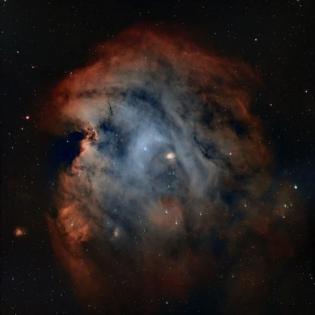
Modern astrophysical exploration relies on unprecedented technological capabilities to unravel the deep mysteries governing our expanding universe. Advanced observatories like the James Webb Space Telescope allow astronomers to peer deeper into the cosmic abyss than ever before. By capturing infrared signatures from ancient celestial formations, scientists can reconstruct the complex lineage of distant cosmic bodies. This genealogical approach to astronomy helps researchers understand how primordial matter evolved into structured star systems and galaxies.

Examining the spectral properties of these newly cataloged objects reveals critical insights regarding early cosmic evolution. Researchers employ rigorous mathematical models and spectroscopic derivations to chart the gravitational and chemical connections linking these remote structures. Each observation acts as a vital data point that refines our broader understanding of cosmic origins and stellar population dynamics. Through meticulous analysis, astrophysicists continue to map the intricate web of interactions shaping the architecture of our universe.

Advanced Spectroscopic Analysis of Distant Astronomical Objects

Unraveling the spectral signatures captured by advanced infrared observatories demands precise mathematical formulation and rigorous data processing. Astronomers utilize sophisticated calibration algorithms to isolate faint signals originating from billions of light-years away. These analytical methods ensure that instrumental noise does not distort the true physical characteristics of the target objects. Consequently, researchers can construct high-fidelity profiles detailing the elemental composition of early cosmic formations.

import numpy as np

import matplotlib.pyplot as plt

def calculate_redshift(observed_wavelength, rest_wavelength):

"""Calculates cosmological redshift based on spectral lines."""

z = (observed_wavelength - rest_wavelength) / rest_wavelength

return z

obs_lambda = 1.216 # micrometers

rest_lambda = 0.1216 # micrometers

redshift_value = calculate_redshift(obs_lambda, rest_lambda)

print(f"Calculated Redshift (z): {redshift_value}")

The mathematical foundation of cosmological redshift provides a direct method for determining the distance and recessional velocity of celestial bodies. By comparing observed spectral line wavelengths with known laboratory reference values, researchers quantify the expansion effects of space-time. The fundamental equation governing this relationship is expressed through precise mathematical parameters.

Further refinement of these calculations involves accounting for relativistic Doppler effects in high-velocity astrophysical environments. When objects exhibit extreme recession speeds, classical approximations fail, requiring strict adherence to relativistic mechanics. The corresponding velocity formulation incorporates the speed of light to maintain absolute analytical precision.

Solving this relativistic expression for velocity yields an accurate metric for tracing galactic trajectories across expansive cosmic distances. Such rigorous derivations empower astrophysicists to model the kinematic history of the universe with extraordinary confidence.

Instrumental Calibration and Photon Detection Paradigms

Infrared detectors aboard space-based telescopes operate at cryogenic temperatures to minimize thermal interference and optimize photon capture efficiency. The primary mirror gathers incoming radiation and focuses it onto highly sensitive focal plane arrays designed for deep space observation. Calibrating these instruments requires correcting for quantum efficiency variations and dark current accumulation across individual pixels.

Mathematical modeling of detector noise ensures that faint astronomical signals remain distinguishable from background instrumental fluctuations. The total signal-to-noise ratio depends heavily on exposure time and aperture collection area. Researchers apply statistical weighting functions to aggregate multiple exposures into a single cohesive dataset.

Optimizing this ratio is essential when examining extremely distant objects whose photon flux diminishes exponentially with distance. Without robust error suppression techniques, crucial spectral features would remain obscured beneath instrumental noise thresholds.

Advanced deconvolution algorithms further enhance spatial resolution by reversing optical aberrations introduced by diffraction limits. These computational procedures rely on point spread function mapping to sharpen blurred astronomical imagery. Through iterative mathematical processing, researchers resolve intricate structural details within distant galactic formations.

Genealogical Classification and Clustering Models

Classifying newly discovered celestial objects requires establishing taxonomic hierarchies based on physical properties, evolutionary status, and spatial clustering. Astronomers map these relationships by analyzing multi-dimensional parameter spaces where each axis represents a distinct observable metric. Hierarchical clustering algorithms group similar entities into distinct families, mirroring biological taxonomy.

Quantitative evaluation of spatial correlation functions helps determine whether distant objects formed through common primordial gas cloud collapses. The two-point correlation function mathematically describes the probability of finding two celestial bodies separated by a specific spatial interval.

Analyzing deviations from homogeneous distributions provides clues regarding dark matter scaffolding and gravitational collapse rates during early epochs. These statistical indicators validate theoretical models of cosmic structure formation.

Machine learning classifiers are increasingly deployed to automate the categorization of millions of transient objects detected by modern sky surveys. Training these models on verified spectroscopic libraries accelerates the discovery pipeline. Consequently, researchers can quickly isolate anomalous formations that challenge existing astrophysical paradigms.

from sklearn.cluster import DBSCAN

import numpy as np

def perform_clustering(feature_matrix):

"""Applies DBSCAN to group celestial objects based on spectral traits."""

clustering = DBSCAN(eps=0.5, min_samples=5).fit(feature_matrix)

return clustering.labels_

mock_data = np.random.rand(100, 3)

labels = perform_clustering(mock_data)

print(f"Assigned cluster labels: {np.unique(labels)}")

The integration of advanced computational tools transforms raw telescopic data into structured genealogical charts of the cosmos. This systematic approach ensures that every newly found distant object is contextualized within the grand tapestry of universal evolution.

Cosmological Evolution and Primordial Lineage Tracking

Reconstructing the lineage of ancient astronomical formations involves tracing their evolutionary pathways back through cosmic time. As light travels across billions of years to reach our detectors, it acts as a historical archive of early stellar processes. Astrophysicists decode this historical record by examining the metallicity gradients and isotopic ratios present in distant systems. These chemical signatures reveal the lifecycle timing of initial stellar generations.

Theoretical models of nucleosynthesis dictate how pristine hydrogen and helium forged heavier elements inside massive primordial stars. When these early stars completed their lifecycles through energetic supernova explosions, they enriched the surrounding interstellar medium. Subsequent generations of stars inherited this enriched material, altering the chemical composition of developing galaxies.

Tracking these metallic variations across different spatial epochs enables researchers to map the genealogical tree of galactic evolution with high fidelity. Each branch of the cosmic tree represents a distinct lineage of stellar assembly and dynamic interaction.

Photometric Redshift Estimation and Spectral Energy Distribution

When high-resolution spectroscopic observations are impractical due to extreme faintness, astronomers rely on photometric redshift estimation techniques. By measuring an object's brightness across multiple broad filters, researchers construct a rough spectral energy distribution curve. Fitting theoretical templates to this curve yields reliable estimates of cosmological distance and stellar mass.

The process involves integrating filter transmission functions with model stellar spectra to predict expected observable magnitudes. Minimizing the chi-squared statistic between observed and template fluxes determines the most probable physical parameters.

This statistical optimization forms the backbone of large-scale census projects examining distant galaxy populations. It bridges the gap between wide-field imaging surveys and targeted spectroscopic confirmation.

import numpy as np

def compute_chi_squared(obs_flux, model_flux, errors, scaling_factor):

"""Computes goodness-of-fit for photometric redshift models."""

residuals = (obs_flux - scaling_factor * model_flux) / errors

return np.sum(residuals ** 2)

flux_o = np.array([10.2, 15.4, 22.1])

flux_m = np.array([9.8, 14.9, 21.0])

errs = np.array([0.5, 0.7, 1.0])

chi2 = compute_chi_squared(flux_o, flux_m, errs, 1.02)

print(f"Computed Chi-Squared: {chi2:.2f}")

Such computational rigor guarantees that statistical inferences drawn from photometric data remain robust against observational uncertainties. Researchers continuously refine these template libraries to accommodate newly discovered classes of celestial objects.

Gravitational Lensing and Mass Distribution Mapping

Massive foreground structures frequently bend the path of light traveling from background sources, producing amplified and distorted images of distant objects. This phenomenon, known as gravitational lensing, acts as a natural magnifying glass that permits the study of objects otherwise too faint to detect. Analyzing the geometric distortions within lensed arcs allows astronomers to map both luminous and dark matter distributions within intermediate clusters.

Reconstructing the gravitational potential requires solving the lens equation, which relates source positions to observed image positions through deflection angles.

In this mathematical framework, ##\beta## represents the true angular position of the background source, ##\theta## denotes the observed image position, and ##\alpha(\theta##) is the deflection angle determined by the mass distribution of the lens.

Inverting this equation to retrieve the underlying mass profile is an ill-posed mathematical problem requiring regularization techniques and parametric modeling. Researchers construct detailed mass maps that reveal the presence of extensive dark matter halos enveloping galaxy clusters.

import numpy as np

def deflection_angle_point_mass(theta, Einstein_radius):

"""Computes deflection angle for a simplistic point-mass lens model."""

alpha = (Einstein_radius ** 2) / theta

return alpha

theta_pos = 1.5 # arcseconds

e_rad = 1.0 # arcseconds

deflection = deflection_angle_point_mass(theta_pos, e_rad)

print(f"Calculated Deflection Angle: {deflection:.3f} arcsec")

Understanding these mass distributions is crucial for evaluating how cosmic structures interact gravitationally across vast cosmological scales. Lensing studies provide independent confirmation of cosmological parameters and dark matter density profiles.

Time Delay Cosmography and Expansion Rate Measurement

When a background source variable object, such as a quasar or supernova, is multiply imaged by a foreground gravitational lens, the light paths travel different geometric distances. Consequently, photons arriving along distinct paths experience measurable time delays. Measuring these time delays provides a direct geometrical method for determining the Hubble constant, independent of traditional local distance ladder calibrations.

The time delay between multiple images combines geometric path length differences with gravitational potential Shapiro time delay effects.

Here, ##D_{\Delta##} represents the time-delay distance, which depends inversely on the expansion rate of the universe. Precision monitoring campaigns track luminosity fluctuations over extended periods to extract robust time delay measurements.

Combining time delay cosmography with stellar kinematic data resolves persistent tensions in modern cosmological measurements. As space telescopes discover more lensed systems, error margins continue to narrow significantly.

Intergalactic Medium Ionization and Reionization Epochs

The epoch of reionization represents a transformative phase transition in cosmological history when neutral hydrogen atoms throughout the intergalactic medium were ionized by energetic ultraviolet radiation from early luminous sources. Space observatories investigate this era by observing the absorption features imprinted on the spectra of distant background objects. Analyzing the Lyman-alpha forest provides a direct probe of neutral hydrogen density fluctuations across intervening space.

The optical depth for resonant scattering by neutral hydrogen atoms along a line of sight at redshift ##z## is governed by specific physical constants and cosmological parameters.

As the universe transitioned from completely neutral to fully ionized, the optical depth decreased markedly, allowing ionizing radiation to propagate freely across intergalactic distances.

Studying these ionization fronts helps researchers identify the primary ionizing agents responsible for clearing the primordial fog. Current consensus points toward a combination of faint star-forming galaxies and active galactic nuclei operating during the first billion years.

def calculate_optical_depth(sigma, neutral_density, path_length):

"""Calculates resonant scattering optical depth."""

return sigma * neutral_density * path_length

sig = 1.6e-17 # cm^2

n_hi = 0.001 # cm^-3

dl = 3.086e24 # cm (1 Mpc)

tau = calculate_optical_depth(sig, n_hi, dl)

print(f"Calculated Optical Depth: {tau:.4f}")

Such calculations link microscopic atomic physics directly to macroscopic cosmological evolution models. The interplay between radiation and gas dynamics dictates the large-scale transparency of the observable universe.

Quasar Probes and Metal Enrichment Timing

Quasars act as luminous background lighthouses whose intense radiation illuminates intervening gas clouds along the line of sight. By analyzing absorption line doublets corresponding to carbon, silicon, and oxygen ions, astronomers determine the metallicity of gas clouds residing in early galactic halos.

The column density ratio of specific ionic species provides a direct diagnostic of ionization parameter and ambient radiation field hardness.

Monitoring these ionic ratios across different redshifts reveals the rapid pace at which early stellar generations dispersed heavy elements into the intergalactic medium.

def compute_ion_ratio(c_iv_column, si_iv_column):

"""Computes ionic column density ratio for metallicity tracing."""

return c_iv_column / si_iv_column

c_val = 1.4e14 # cm^-2

si_val = 4.2e13 # cm^-2

ratio = compute_ion_ratio(c_val, si_val)

print(f"Computed Ion Ratio: {ratio:.2f}")

These empirical findings support models of vigorous early star formation followed by galactic-scale outflows that redistributed enriched gas far beyond visible stellar boundaries.

Computational Astrophysics and Big Data Pipeline Integration

Modern space observatories generate petabytes of raw observational data that require automated processing pipelines before scientific analysis can begin. Computational astrophysics bridges the gap between raw photon counts and published theoretical discoveries. Automated calibration routines remove instrumental artifacts, cosmic ray hits, and scattered light contamination from every exposure.

Parallel processing clusters distribute heavy computational workloads across thousands of CPU and GPU cores to execute complex ray-tracing and radiative transfer simulations.

Optimizing parallel execution efficiency is vital for managing the exponential growth of astronomical datasets generated by next-generation observatories.

Cloud-based data archives provide global research teams with instantaneous access to calibrated catalogs, enabling collaborative exploration on an unprecedented international scale.

Machine Learning in Automated Anomaly Detection

With millions of celestial objects cataloged in public surveys, manual inspection becomes impossible. Deep learning architectures, particularly convolutional neural networks and unsupervised autoencoders, are deployed to scan image repositories for rare anomalies, such as Einstein rings, colliding galaxies, or primordial stellar nurseries.

Unsupervised models learn representations of normal galaxy morphologies without requiring labeled training sets, allowing them to isolate statistical outliers that deviate significantly from standard population trends.

Minimizing reconstruction loss trains the autoencoder to faithfully compress and decompress typical galactic profiles, flagging abnormal residuals for expert human review.

import tensorflow as tf

from tensorflow.keras import layers, models

def build_autoencoder(input_shape):

"""Constructs a convolutional autoencoder for anomaly detection."""

model = models.Sequential([

layers.Input(shape=input_shape),

layers.Conv2D(16, (3, 3), activation='relu', padding='same'),

layers.MaxPooling2D((2, 2), padding='same'),

layers.Conv2D(16, (3, 3), activation='relu', padding='same'),

layers.UpSampling2D((2, 2))

])

return model

ae_model = build_autoencoder((64, 64, 1))

ae_model.compile(optimizer='adam', loss='mse')

print("Autoencoder model successfully compiled for astronomical anomaly detection.")

These intelligent screening systems ensure that groundbreaking discoveries are identified and prioritized immediately upon data downlink.

Future Horizons in Deep Space Exploration and Observational Cosmology

The ongoing success of space-based infrared observatories paves the way for even more ambitious astronomical missions designed to probe the earliest moments of cosmic history. Future space telescopes will feature larger primary mirrors and enhanced spectroscopic bandwidths, enabling astronomers to resolve individual stars within galaxies located near the edge of the observable universe. These technological advancements promise to resolve lingering questions concerning dark energy, cosmic inflation, and galaxy assembly mechanics.

International collaboration remains paramount as the astronomical community designs next-generation instrumentation to tackle complex observational challenges. By combining space-based infrared data with ground-based radio and optical surveys, researchers achieve a multi-messenger perspective on universal evolution.

Maintaining precise closure equations across cosmological parameters validates our foundational understanding of space-time geometry and mass-energy distribution.

As new distant objects are uncovered and their genealogical connections mapped, humanity edges closer to comprehending the full chronological narrative of the cosmos.

The Role of Citizen Science in Astronomical Discovery

While professional pipelines and machine learning algorithms process massive volumes of telescopic data, human pattern recognition remains exceptionally valuable for identifying complex morphological structures that automated routines might overlook. Citizen science platforms allow enthusiasts worldwide to participate directly in classifying galaxy shapes, searching for gravitational lenses, and flagging stellar transients.

Integrating crowdsourced classifications with professional machine learning models creates a powerful hybrid discovery framework. This participatory approach broadens public engagement with cutting-edge science while expanding the analytical capacity of modern astronomical research initiatives.

def aggregate_citizen_classifications(user_votes):

"""Calculates weighted consensus score from volunteer classifications."""

consensus = sum(user_votes) / len(user_votes)

return consensus

votes = [1, 1, 0, 1, 1, 1, 0, 1]

score = aggregate_citizen_classifications(votes)

print(f"Aggregated Consensus Score: {score:.2f}")

Empowering global participants ensures that the wonders of deep space exploration remain accessible to everyone, fostering a universal appreciation for the scientific endeavor.