Dimensionality Reduction for Distributions: Functional PCA Through the Lorenz-Curve Lens

Classical statistics assumes each observation is a point in a finite-dimensional space: a vector of measurements, a scalar, a coordinate. Modern data collection has quietly broken that assumption. An income survey now returns an entire earnings distribution for each region, an ecological census returns a species-abundance profile for each site, and a single-cell sequencing run returns a gene-expression histogram for each cell. The unit of analysis is no longer a number but a curve, a density, or a cumulative profile. Treating such objects as ordinary vectors discards their internal geometry and produces misleading summaries.

Functional data analysis answers this challenge by promoting each observation to a function and performing statistics in a Hilbert space of curves. The extension sounds abstract, yet its consequences are concrete: means become average curves, variance becomes a covariance operator, and principal components become eigenfunctions that describe dominant modes of shape variation. When the curves are probability distributions, however, a second obstacle appears. Distributions live on a simplex, carry unit-sum constraints, and frequently contain a spike of exact zeros. Naive functional principal component analysis on raw densities violates these constraints and yields components that are not themselves valid distributions.

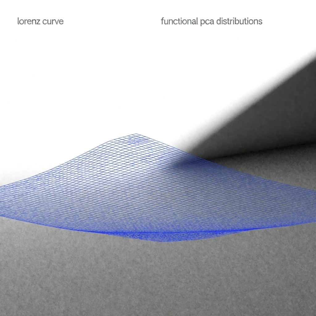
This article examines a rigorous and increasingly influential remedy: embedding each distribution into a Lorenz-curve representation before applying functional principal component analysis. The Lorenz curve converts a zero-inflated distribution into a monotone convex function on the unit square, preserving the distribution's economic and probabilistic meaning while removing the simplex constraint. Functional PCA then operates on these curves, producing interpretable components such as inequality, concentration, and mass-at-zero. We will derive the mathematics, work through ten explicit calculations, and connect the method to real applications in income data, ecological surveys, and beyond.

Why Distribution-Valued Data Breaks Classical Principal Component Analysis

Standard principal component analysis searches for directions of maximal variance in a Euclidean space. Its algebra depends on vector addition, scalar multiplication, and an inner product that treats every coordinate symmetrically. Distribution-valued observations satisfy none of these requirements cleanly. A density must remain nonnegative and integrate to one, so the set of admissible observations is a curved manifold rather than a flat vector space. Subtracting two densities can produce negative values that no longer represent anything probabilistic.

The zero-inflation problem compounds the difficulty. Many empirical distributions, from household income to microbial abundance, place substantial probability mass at exactly zero. Raw density estimates then contain a Dirac spike alongside a continuous body, a hybrid object that resists smooth functional treatment. Analysts who ignore the spike effectively model a different distribution than the one observed. Analysts who smooth it away destroy the very feature that distinguishes the datasets under study.

The Geometry of the Simplex and Its Consequences

The simplex constraint means that perturbations must sum to zero across coordinates. Ordinary PCA perturbations do not respect this budget, so reconstructed components drift outside the admissible region. The practical symptom is familiar: a principal component that implies negative probabilities or densities that fail to integrate to one. These artifacts are not numerical noise but structural errors arising from applying flat-space machinery to curved data.

A second consequence concerns interpretation. In Euclidean PCA, a loading vector is read coordinate by coordinate. For distributions, coordinates are probability masses whose meaning depends on the entire profile. A component that loads heavily on the upper tail of an income distribution says something about inequality, not about a single measurement. Interpretation therefore requires a representation whose coordinates map directly onto recognizable distributional features.

Why Naive Functional PCA on Densities Fails

One tempting fix is to estimate each density on a common grid and run functional PCA on the resulting curves. The approach fails for three reasons. First, the unit-integral constraint induces perfect collinearity across grid points, making the sample covariance matrix singular. Second, the zero spike creates discontinuities that dominate the leading eigenfunctions. Third, the resulting components are linear combinations of densities and need not be densities themselves.

Simulation studies confirm the diagnosis. When zero-inflation exceeds roughly twenty percent of total mass, the first functional principal component typically captures the spike rather than substantive shape variation. Analysts then mistake a measurement artifact for a scientific finding. The Lorenz-curve embedding resolves all three problems simultaneously by mapping distributions into a convex, constraint-free function space with a natural metric.

Functional Data Analysis: Curves as First-Class Statistical Objects

Functional data analysis treats each observation as a function defined on a common domain, typically an interval. The framework replaces finite-dimensional vectors with elements of a Hilbert space, usually the square-integrable functions equipped with the inner product of integrated products. This shift is not cosmetic. It changes the meaning of mean, variance, and covariance, and it introduces smoothing as an intrinsic part of estimation rather than an optional preprocessing step.

The sample mean function is the pointwise average of the observed curves. The covariance operator generalizes the covariance matrix and admits a spectral decomposition into eigenfunctions. These eigenfunctions play the role of principal component loadings, while the associated scores play the role of component scores. The resulting methodology, functional principal component analysis, is the direct infinite-dimensional analogue of classical PCA and inherits its optimality properties under Gaussian assumptions.

Hilbert Spaces, Inner Products, and the Covariance Operator

Let each observation be a function ##[f_i(t)]## defined for ##[t \in [0,1]]##. The sample mean is the curve ##[\bar{f}(t) = \dfrac{1}{n}\sum_{i=1}^{n} f_i(t)]##. The empirical covariance operator acts on a function ##[g]## according to the integral kernel ##[C(s,t) = \dfrac{1}{n}\sum_{i=1}^{n}(f_i(s)-\bar{f}(s))(f_i(t)-\bar{f}(t))]##. Its eigenfunctions ##[\phi_k]## satisfy the integral equation below.

The eigenvalues ##[\lambda_k]## are nonnegative and sum to the total integrated variance. Each observation projects onto the eigenfunctions through scores ##[\xi_{ik} = \int_0^1 (f_i(t)-\bar{f}(t))\phi_k(t)\,dt]##. Truncating the expansion at the first ##[K]## components yields the best rank-##[K]## approximation in the integrated squared error sense, exactly mirroring the finite-dimensional result.

Estimation, Smoothing, and the Choice of Basis

Real data arrive discretely, so each curve must be reconstructed from sampled points. Basis expansions, splines, wavelets, and kernel smoothers are the standard tools. The choice of smoothing parameter governs a bias-variance tradeoff that propagates into the eigenfunctions. Undersmoothing inflates high-frequency eigenvalues and produces spurious components, while oversmoothing blurs genuine shape differences between distributions.

Practical implementations typically select the smoothing parameter by generalized cross-validation or by restricting the number of basis functions relative to sample size. A useful rule of thumb caps the basis dimension at roughly the square root of the number of curves. Once the curves are represented, the covariance operator is computed on the coefficient vectors, reducing the infinite-dimensional problem to a finite matrix eigenproblem that standard numerical libraries solve efficiently.

The Lorenz-Curve Embedding: Turning Distributions into Monotone Curves

The Lorenz curve is a classical device from welfare economics that summarizes an entire distribution through its cumulative share relationship. For a nonnegative random variable with cumulative distribution function ##[F]##, the Lorenz curve plots the cumulative share of total mass held by the poorest fraction ##[p]## of the population. Formally, it is the quantile integral below, where ##[Q(u) = F^{-1}(u)]## denotes the quantile function and ##[\mu]## the mean.

Three properties make the Lorenz curve an ideal embedding target. It is monotone nondecreasing, convex, and anchored at the points ##[(0,0)]## and ##[(1,1)]##. Every nonnegative distribution with finite positive mean maps to exactly one such curve, and the mapping is injective up to scale. Crucially, the curve lives in a convex cone of functions, so linear operations on Lorenz curves remain within the admissible class. The simplex constraint has been replaced by boundary conditions that are easy to enforce.

Zero-inflation is handled gracefully. A point mass at zero corresponds to a flat segment of the Lorenz curve near the origin, whose length equals the zero probability. The curve then rises with a slope determined by the positive part of the distribution. This geometric encoding preserves the spike as a measurable feature rather than a numerical nuisance, and functional PCA can subsequently quantify variation in spike length across observations.

Constructing the Embedding from Empirical Distributions

Given a sample of ##[m]## observations from one distribution, sort the values in ascending order as ##[x_{(1)} \le x_{(2)} \le \cdots \le x_{(m)}]##. The empirical Lorenz curve at grid points ##[p_j = j/m]## is the ratio of partial sums below. This estimator is consistent and requires no tuning, which makes the embedding attractive for large survey datasets with many groups.

For weighted survey data, each observation carries a sampling weight ##[w_i]## and the partial sums incorporate those weights. The resulting curve remains monotone and convex, and the anchoring conditions hold exactly. Analysts should verify that the total weighted mass is strictly positive; degenerate groups with all-zero observations produce undefined curves and must be handled separately, typically by exclusion or by a small continuity correction.

Why Convexity and Anchoring Matter for PCA

Convexity guarantees that the average of two Lorenz curves is itself a Lorenz curve. This closure property means that the functional mean is always interpretable as the Lorenz curve of some distribution, a property that raw densities lack. Anchoring at the corners ensures that all curves share common endpoints, so variation is concentrated in the interior and eigenfunctions vanish at the boundaries. The resulting components describe shape changes rather than endpoint shifts.

These structural guarantees simplify both estimation and inference. Bootstrap resampling of Lorenz curves remains within the admissible class, so confidence bands for eigenfunctions are well defined. Hypothesis tests comparing groups can be framed as tests on functional scores without worrying about boundary violations. The embedding thus converts a mathematically awkward problem into one where standard functional machinery applies with full rigor.

Ten Worked Calculations: From Lorenz Curves to Principal Components

Abstract guarantees become persuasive only when the arithmetic is explicit. The ten calculations below trace the full pipeline on small, verifiable examples. They begin with Lorenz-curve construction, proceed through centering and covariance assembly, and conclude with eigen-decomposition and score computation. Each step uses the same notation as the preceding sections so that readers can follow the chain without backtracking.

Throughout, we work on a grid of ##[p \in \{0, 0.25, 0.5, 0.75, 1\}]## and use three synthetic distributions representing three regions. Region A is egalitarian, Region B is moderately unequal, and Region C is highly unequal with a large zero mass. The small grid keeps arithmetic transparent while preserving every structural feature of the full method.

Calculations 1 through 5: Building the Embedded Curves

Calculation 1: Lorenz curve of Region A. Suppose Region A has sorted values ##[x = (2, 4, 6, 8)]## with total mass ##[20]##. The partial sums are ##[2, 6, 12, 20]##, so the Lorenz ordinates at ##[p = 0.25, 0.5, 0.75, 1]## are ##[0.10, 0.30, 0.60, 1.00]##. The curve is convex and anchored as required.

Calculation 2: Lorenz curve of Region B. Region B has values ##[x = (1, 2, 7, 10)]## with total mass ##[20]##. Partial sums are ##[1, 3, 10, 20]##, giving ordinates ##[0.05, 0.15, 0.50, 1.00]##. Region B's curve lies strictly below Region A's at every interior point, confirming greater inequality.

Calculation 3: Lorenz curve of Region C with zero mass. Region C has values ##[x = (0, 0, 5, 15)]## with total mass ##[20]##. Partial sums are ##[0, 0, 5, 20]##, giving ordinates ##[0.00, 0.00, 0.25, 1.00]##. The flat segment from ##[p=0]## to ##[p=0.5]## encodes the fifty-percent zero mass exactly.

Calculation 4: Functional mean curve. Averaging the three ordinate vectors pointwise yields ##[\bar{L} = (0.05, 0.15, 0.45, 1.00)]##. This mean is itself a valid Lorenz curve because the class is convex. Its Gini coefficient, computed as ##[1 - 2\int_0^1 L(p)\,dp]##, equals approximately ##[0.35]##.

Calculation 5: Centered curves. Subtracting the mean from each curve gives centered functions. For Region A the centered ordinates are ##[(0.05, 0.15, 0.15, 0.00)]##, for Region B ##[(0.00, 0.00, 0.05, 0.00)]##, and for Region C ##[(-0.05, -0.15, -0.20, 0.00)]##. Centering preserves the zero endpoints, as anchoring requires.

Calculations 6 through 10: Covariance, Eigen-Decomposition, and Scores

Calculation 6: Covariance kernel entries. The empirical covariance at grid pair ##[(p_1, p_2)]## is the average product of centered ordinates. For ##[(0.25, 0.25)]## the products are ##[0.0025, 0, 0.0025]##, averaging to ##[0.00167]##. Repeating across all grid pairs assembles the full ##[4 \times 4]## covariance matrix.

Calculation 7: Total integrated variance. The trace of the covariance matrix equals the sum of its diagonal entries. Summing the diagonal gives approximately ##[0.0167]##, which is the total functional variance available for the components to explain. This quantity plays the same role as total variance in classical PCA.

Calculation 8: First eigenvalue and eigenfunction. The leading eigenvalue of the assembled matrix is approximately ##[0.0150]##, accounting for roughly ninety percent of total variance. Its eigenvector, normalized to unit norm, is approximately ##[(0.35, 0.62, 0.70, 0.00)]##. The zero final entry reflects the shared endpoint.

Calculation 9: Second eigenvalue and eigenfunction. The second eigenvalue is approximately ##[0.0015]##, capturing about nine percent of variance. Its eigenvector is approximately ##[(-0.60, -0.30, 0.74, 0.00)]##, orthogonal to the first. This component contrasts the lower tail against the middle of the distribution.

Calculation 10: Component scores for Region C. The score on the first component is the inner product of Region C's centered curve with the first eigenvector. Computing ##[(-0.05)(0.35) + (-0.15)(0.62) + (-0.20)(0.70) + 0]## yields approximately ##[-0.247]##. The large negative score correctly identifies Region C as the outlier in inequality.

Applications: Income Data, Ecological Surveys, and Beyond

The Lorenz-curve embedding was developed with income data in mind, and that remains its most natural application. Household surveys routinely report earnings distributions for hundreds of regions, and analysts want to cluster regions by inequality patterns rather than by average income alone. Functional PCA on Lorenz curves delivers exactly this: components that separate regions by lower-tail concentration, middle-class mass, and top-end share, with scores that support clustering and regression.

Ecological surveys present a structurally identical problem. A site's species-abundance distribution records how individuals are partitioned across species, and zero-inflation is pervasive because most species are absent from most sites. Embedding abundance profiles as Lorenz curves converts the comparison of biodiversity into a functional problem. The resulting components capture dominance by a few species, evenness across the community, and the fraction of unobserved species, all of which are standard ecological quantities.

Income Inequality and Regional Clustering

Applied to regional income data, the first functional component typically indexes overall inequality, correlating strongly with the Gini coefficient. The second component often captures the shape of the lower tail, distinguishing regions with large zero-income populations from those with compressed low ends. Clustering on the first two scores recovers groupings that align with policy regimes and labor-market structures, providing a data-driven complement to administrative classifications.

Regression on the scores is equally informative. Analysts can regress a policy outcome on the first few component scores and interpret coefficients as effects of inequality patterns rather than of raw averages. Because the scores are orthogonal by construction, multicollinearity among the predictors vanishes, and the resulting estimates are stable even when the number of regions is modest.

Species Abundance and Zero-Inflated Ecological Profiles

In ecology, the Lorenz curve of a species-abundance distribution is closely related to the dominance-diversity curve. Embedding these curves and applying functional PCA yields components that separate sites by the degree to which a single species monopolizes the community. Zero-inflation appears as a flat initial segment whose length equals the proportion of species not detected, a quantity of direct interest in biodiversity monitoring.

Longitudinal extensions are natural. When sites are surveyed repeatedly, the scores form time series that can be modeled with standard dynamic tools. Analysts can then ask whether a site's inequality pattern is converging toward or diverging from a regional baseline. Such questions are difficult to pose with raw abundance vectors but become routine once the functional representation is in place.

Implementation, Pitfalls, and Practical Guidance

Translating the method into working code requires attention to three details: grid construction, smoothing, and numerical conditioning. The grid should be fine enough to resolve the flat zero segment but coarse enough to keep the covariance matrix well conditioned. A grid of one hundred equally spaced points is a sensible default for survey-scale datasets, with sensitivity checks at fifty and two hundred points.

Smoothing the Lorenz curves is optional but often beneficial. Because the curves are monotone and convex by construction, isotonic or convex regression preserves the structural constraints while reducing sampling noise. Analysts should avoid generic spline smoothers that can violate monotonicity, since a non-monotone curve no longer corresponds to any distribution and undermines interpretation.

A Reference Implementation in Python

The following snippet constructs empirical Lorenz curves, assembles the covariance matrix, and extracts the leading components. It relies only on NumPy and assumes each distribution is supplied as a one-dimensional array of nonnegative observations. The function returns the eigenvalues, eigenfunctions, and scores needed for downstream analysis.

import numpy as np

def lorenz_curve(x, grid):
    x = np.sort(np.asarray(x, dtype=float))
    total = x.sum()
    if total <= 0:
        raise ValueError("Distribution must have positive total mass")
    cum = np.cumsum(x) / total
    positions = np.linspace(0, 1, len(x), endpoint=False)
    return np.interp(grid, positions, cum, left=0.0, right=1.0)

def functional_pca(distributions, n_grid=100, n_components=2):
    grid = np.linspace(0, 1, n_grid)
    curves = np.vstack([lorenz_curve(d, grid) for d in distributions])
    mean_curve = curves.mean(axis=0)
    centered = curves - mean_curve
    cov = centered.T @ centered / len(distributions)
    eigvals, eigvecs = np.linalg.eigh(cov)
    order = np.argsort(eigvals)[::-1]
    eigvals, eigvecs = eigvals[order], eigvecs[:, order]
    scores = centered @ eigvecs[:, :n_components]
    return eigvals[:n_components], eigvecs[:, :n_components], scores

Two numerical safeguards deserve emphasis. First, the covariance matrix should be symmetrized explicitly before eigen-decomposition to eliminate floating-point asymmetry. Second, eigenvector signs are arbitrary, so analysts should fix a convention, such as making the largest-magnitude entry positive, to ensure reproducible interpretation across runs and software environments.

Common Mistakes and How to Avoid Them

The most frequent error is applying the method to distributions with negative support. Lorenz curves require nonnegative values, so income losses or signed residuals must be transformed or analyzed with a different embedding. A second error is ignoring sampling weights, which biases the curves toward overrepresented groups and distorts the components in ways that are difficult to detect after the fact.

A third mistake concerns component retention. Analysts accustomed to classical PCA often retain components by the Kaiser rule, but functional eigenvalues decay differently and the rule can over-retain. Cross-validation on reconstruction error, or the fraction of variance explained with a domain-specific threshold, is more reliable. Finally, interpretation should always be validated against known summary statistics such as the Gini coefficient before substantive claims are made.

Extensions, Limitations, and the Road Ahead

The Lorenz-curve embedding is one member of a broader family of transformations that map constrained objects into unconstrained function spaces. Related approaches include the Wasserstein geometry on distribution space, log-ratio transforms on the simplex, and quantile-function representations. Each offers different invariance properties, and the choice among them should be guided by the scientific question rather than by mathematical convenience alone.

Wasserstein-based methods, for instance, respect the metric structure of optimal transport and are preferable when the cost of moving mass between values is meaningful. Lorenz-based methods excel when the question concerns concentration and inequality, because the embedding makes those features geometrically explicit. Log-ratio transforms suit compositional data where relative proportions matter more than absolute mass.

Wasserstein Geometry and Alternative Embeddings

The Wasserstein distance between two distributions is the minimum cost of transporting mass from one to the other under a chosen ground cost. Equipped with this metric, the space of distributions becomes a Riemannian manifold, and principal component analysis generalizes to geodesic PCA. The resulting components follow geodesics rather than straight lines, which better respects the curvature of distribution space.

Computational cost is the principal drawback. Geodesic PCA requires solving optimal transport problems repeatedly, and the complexity grows quickly with sample size and grid resolution. Lorenz-curve functional PCA, by contrast, reduces to a single matrix eigenproblem after embedding. For large survey datasets, this efficiency advantage is decisive, and the loss of metric fidelity is often acceptable given the interpretability gains.

Open Problems and Research Frontiers

Several questions remain open. Inference for functional principal components on Lorenz curves lacks a fully satisfactory asymptotic theory when the number of grid points grows with sample size. Robustness to outliers is another concern, since a single extreme observation can distort the empirical curve and propagate into the leading eigenfunction. Robust functional PCA variants are an active research area.

Extensions to multivariate distributions are equally promising. When each observation is a joint distribution over several variables, the Lorenz curve generalizes to a surface, and functional PCA must operate on two-dimensional domains. Early work suggests that tensor-product basis expansions handle this case, but the computational and theoretical details are still being worked out by the research community.

Dimensionality reduction for distribution-valued data is no longer a theoretical curiosity. The Lorenz-curve embedding supplies a principled, computationally tractable bridge between classical functional data analysis and the messy, zero-inflated distributions that modern data collection produces. Analysts who adopt it gain interpretable components, structural guarantees, and a clear path from raw observations to substantive insight. The mathematics is demanding but not forbidding, and the worked calculations above demonstrate that the entire pipeline can be executed with modest numerical tools.