The Hidden Mathematics of Tennis: Modeling Every Rally as a Markov Chain

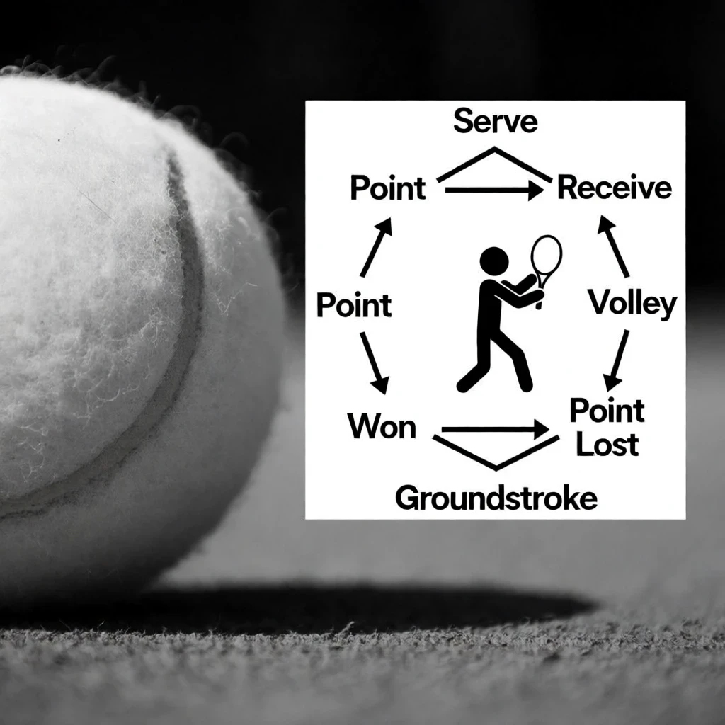
A tennis point looks like chaos when you watch it at full speed: a serve, a scrambling return, a cross-court exchange, then a sudden winner down the line. Yet beneath that apparent disorder lies a remarkably structured system of decisions, each one constrained by geometry, fatigue, and the opponent's anticipation. Probability theory gives us the language to describe that structure precisely, and the Markov chain is its most elegant instrument. By treating each shot location as a state and each subsequent shot as a transition, analysts convert a fleeting athletic contest into a measurable, predictive machine.

This framework matters far beyond the tennis court. Markov models power search engines, speech recognition, credit scoring, and weather forecasting, so a familiar game becomes an accessible doorway into genuinely advanced statistics. Readers who have never encountered a transition matrix can grasp its logic through a forehand struck repeatedly to the same corner. The sport supplies intuition; the mathematics supplies rigor. Together they reveal tactical patterns that conventional win–loss summaries simply cannot capture, no matter how detailed the box score appears.

What follows is a complete treatment of the shot-location transition model: how states are defined, how probabilities are estimated, how stationary distributions expose strategic equilibrium, and how the resulting numbers translate into coaching insight. Expect concrete calculations, real interpretive depth, and a clear demonstration that probability is not an abstraction hovering above sport but the hidden grammar of every rally.

Why a Tennis Point Behaves Like a Stochastic Process

A stochastic process is any system that evolves through time according to probabilistic rules, and a tennis rally fits that definition with unusual precision. Each shot occupies a discrete location, each transition depends only on the current situation, and the sequence terminates when a point is won or lost. The rally therefore unfolds as a chain of conditional probabilities rather than a scripted sequence.

Defining the State Space of a Rally

The first modeling decision is granularity. Analysts typically divide the court into a grid of zones, often three depth bands crossed with three lateral bands, producing nine states per side. A shot landing in the deep deuce corner becomes a single symbol, and the model tracks movement between symbols rather than continuous coordinates.

Finer grids capture more tactical nuance but demand exponentially more data before estimates stabilize. Coarse grids generalize quickly yet blur distinctions between, say, a deep cross-court forehand and a short angled one. The art lies in choosing a resolution that matches both the available tracking data and the strategic question being asked.

Modern optical tracking systems record ball position dozens of times per second, so raw data is rarely the constraint. The real limitation is sample size per transition: rare patterns like serve-plus-volley combinations occur infrequently enough that their probabilities carry wide confidence intervals. Prudent modelers pool data across matches or players to stabilize estimates.

Once states are fixed, the rally becomes a walk through a directed graph. Nodes represent locations, edges represent possible next shots, and edge weights represent transition frequencies. This graph is the Markov chain's skeleton, and every subsequent calculation reads directly from it.

The Markov Property and Its Tennis Interpretation

The Markov property asserts that the future depends only on the present state, not on the path taken to reach it. In tennis terms, the probability of the next shot depends on where the ball currently is, not on the three shots that preceded it. This assumption is powerful and imperfect.

Strictly speaking, momentum and fatigue violate memorylessness: a player who has sprinted through five long exchanges behaves differently from one fresh at the start of a point. Yet empirical work shows the approximation holds well enough for tactical analysis, especially when player identity and rally length are included as auxiliary variables.

Formally, the model states that the conditional probability of the next location depends only on the current one. Written compactly, the transition probability from state ##[i]## to state ##[j]## is ##[P_{ij} = \Pr(X_{t+1} = j \mid X_t = i)]##, and the full collection of these values forms the transition matrix that governs the entire rally.

This memoryless structure is precisely what makes the model tractable. Instead of simulating every historical contingency, analysts multiply matrices and read off long-run behavior. The simplification buys enormous analytical power at a modest cost in realism.

Constructing the Transition Matrix from Shot Data

Building the matrix is an exercise in careful counting. Every observed shot contributes one transition from its landing zone to the next shot's landing zone, and dividing row counts by row totals yields empirical probabilities. The resulting matrix is a compact fingerprint of a player's tactical identity, readable at a glance once you know how to interpret its rows.

Estimating Probabilities from Observed Rallies

Suppose a player hit 240 shots from the deep cross-court zone and 96 of them went to the deep down-the-line zone. The maximum-likelihood estimate for that transition is simply ##[P = \dfrac{96}{240} = 0.40]##, a clean ratio that requires no sophisticated machinery to compute or defend.

Raw frequencies, however, can mislead when counts are small. A transition observed only four times might show a probability of 0.75 purely by chance. Bayesian smoothing, which adds small pseudo-counts to every cell, tempers these extremes and produces estimates that behave sensibly in sparse regions of the matrix.

Consider a simplified three-state model with zones labeled Cross, Middle, and Line. A plausible empirical matrix might place 0.55 on staying cross-court, 0.30 on shifting to the middle, and 0.15 on redirecting down the line, values consistent with the conservative patterns seen in professional baseline exchanges.

Each row must sum to one, a constraint that reflects the certainty that some shot follows every shot. Verifying row sums is the first sanity check any analyst performs, and violations almost always signal a data-processing error rather than a genuine anomaly.

Reading Strategy Directly from Matrix Rows

A row of the transition matrix is a strategic confession. High diagonal entries indicate repetition and patience; large off-diagonal entries reveal aggression and risk-taking. Comparing rows across players exposes stylistic differences that raw winners-and-errors counts flatten into indistinguishability.

Consider two players with identical win rates but opposite matrices. One grinds from the cross-court corner with 0.70 persistence, while the other redirects down the line 0.35 of the time. The first player's strategy is attritional, the second's is predatory, and only the matrix distinguishes them.

Coaches can exploit this directly. If an opponent's matrix shows a strong tendency to redirect under pressure, the scouting report becomes a specific instruction: anticipate the line change on the third shot of cross-court exchanges. The probability model converts observation into actionable preparation.

Rows also evolve within a match. A player losing the first set may shift probabilities toward higher-variance patterns, and tracking that drift in real time offers a quantitative window into tactical adjustments that commentary usually describes only impressionistically.

Computing Multi-Shot Probabilities Through Matrix Powers

Single-step transitions describe the next shot, but strategy unfolds over several shots. Matrix multiplication answers the deeper question: given the current location, what is the probability of reaching a particular zone three shots from now? The answer lives in the corresponding entry of the squared or cubed matrix.

Worked Calculation of a Two-Step Transition

Take the Cross row of our matrix and ask for the probability of returning to Cross after two shots. The chain can pass through any intermediate state, so we sum the products along each possible path, a calculation that directly embodies the law of total probability.

The arithmetic proceeds as follows, multiplying each first-step probability by the corresponding second-step probability and adding the three contributions together. This single number summarizes a compound tactical event that would otherwise require careful enumeration of every route.

The result, roughly 0.475, is lower than the one-step value of 0.55 because the chain can wander into the Middle or Line zones before returning. Multi-step probabilities generally decay toward the stationary distribution, a phenomenon we examine shortly.

Extending to three steps requires multiplying the squared matrix by the original once more. The computation grows tedious by hand but trivial for software, and the resulting entries quantify how quickly a player's tactical tendencies converge toward long-run equilibrium.

Absorbing States and Point Termination

Rallies end, and the model must account for termination. Analysts add absorbing states representing point won and point lost, with transitions from every location into these terminal states. The augmented matrix then yields the probability of winning from any starting position.

This construction is standard absorbing-chain theory. If ##[Q]## is the submatrix of transitions among transient locations and ##[R]## the submatrix of transitions into terminal states, then the fundamental matrix ##[N = (I - Q)^{-1}]## gives expected visits to each transient state before absorption.

The win probability from a starting state follows from multiplying the fundamental matrix by the absorption probabilities. In compact form, the vector of win probabilities is ##[\mathbf{w} = N R_{\text{win}}]##, where ##[R_{\text{win}}]## collects the probabilities of transitioning directly into the winning state.

These calculations transform vague tactical intuition into precise expected values. A coach can now state that a particular serve pattern raises the point-win probability from 0.58 to 0.64, a claim grounded in matrix algebra rather than anecdote.

Stationary Distributions and Long-Run Tactical Equilibrium

If a player repeated rallies indefinitely under fixed transition rules, the distribution of shot locations would settle into a stable pattern called the stationary distribution. This vector satisfies the elegant equation ##[\boldsymbol{\pi} P = \boldsymbol{\pi}]##, meaning the distribution reproduces itself after every shot.

Solving for the Equilibrium Vector

Finding the stationary distribution amounts to solving a small linear system alongside the normalization constraint that probabilities sum to one. For our three-state matrix, the solution reveals which zones dominate a player's long-run shot mix, independent of where the rally began.

The equations are straightforward to set up and solve by substitution. Each component of the stationary vector equals the weighted sum of transitions into that state, and the normalization condition closes the system with a unique solution for an irreducible chain.

Solving the full system yields approximate equilibrium values of 0.48 for Cross, 0.33 for Middle, and 0.19 for Line. These proportions describe the player's characteristic shot diet once transient effects fade, a signature as distinctive as a fingerprint.

Deviations from equilibrium are diagnostically interesting. A player whose observed shot mix departs sharply from the stationary prediction may be executing an intentional tactical shift, or may simply be losing points before the chain converges.

Interpreting Equilibrium as Strategic Identity

The stationary distribution is best read as a player's default tactical identity. A high equilibrium weight on the cross-court zone signals a grinder who builds points patiently; a substantial line weight signals an aggressor who seeks early termination through risk.

Comparing stationary vectors across opponents also informs matchup analysis. If one player's equilibrium concentrates in zones where the opponent's defensive transitions are weakest, the model predicts exploitation, and the prediction is testable against historical head-to-head data.

Equilibrium analysis further reveals why stylistic clashes produce predictable patterns. Two grinders facing each other generate long cross-court exchanges, while an aggressor against a grinder produces short, volatile rallies whose outcome hinges on the aggressor's conversion rate.

These insights remain invisible in conventional statistics. Winners and unforced errors record outcomes, but the stationary distribution records the process that generates them, and process knowledge is what actually guides tactical preparation.

What the Model Reveals That Box Scores Conceal

Conventional tennis statistics count outcomes: aces, double faults, winners, unforced errors. These numbers describe what happened but say nothing about how. The transition model inverts the emphasis, describing the generative process that produces outcomes and thereby explaining why two players with identical totals can be tactically opposite.

Beyond Winners and Unforced Errors

Consider two players each recording 30 winners and 25 unforced errors in a match. The box score declares them equivalent, yet one may have built points through patient cross-court construction while the other gambled on low-percentage line changes. Only transition data separates them.

The model also quantifies shot quality in context. A down-the-line backhand executed from a neutral position carries different strategic weight than the same shot struck from a defensive scramble, and transition probabilities conditioned on prior location capture that distinction naturally.

Pressure effects become measurable as well. By comparing transition matrices in break points against those in routine games, analysts can test whether players genuinely tighten or whether the perception of choking is a narrative artifact unsupported by data.

These comparisons require careful statistical hygiene. Confidence intervals around transition probabilities, computed via bootstrap resampling, prevent analysts from overinterpreting small differences that could easily arise from sampling noise alone.

Practical Applications in Coaching and Broadcasting

Coaching staffs increasingly use transition models to design practice sessions. If a player's matrix shows weak conversion from the middle zone, drills can target that specific transition until the probability improves, creating a measurable feedback loop between analysis and training.

Broadcasters benefit from the same machinery. On-screen graphics showing live transition tendencies give viewers a quantitative layer beneath the commentary, explaining why a particular pattern keeps recurring and what the players are likely to attempt next.

Betting markets and fantasy platforms incorporate these models to sharpen pricing. A serve pattern with a demonstrably higher point-win probability should shift the odds, and models that ignore transition structure systematically misprice such advantages.

Player development pathways use the framework longitudinally. Tracking a junior's transition matrix across seasons reveals whether tactical maturity is developing, offering objective evidence where subjective scouting reports once dominated the evaluation.

Limitations, Extensions, and the Road Ahead

No model is a mirror, and the Markov chain simplifies tennis in ways that matter. Memorylessness ignores momentum, fixed transition probabilities ignore adaptation, and discrete zones ignore the continuous geometry of the court. Acknowledging these limits is not a concession but a precondition for honest analysis.

Where the Markov Assumption Breaks Down

Momentum is the most conspicuous violation. A player who wins three consecutive points may genuinely play differently on the fourth, which means the transition probabilities depend on history rather than solely on current location. Hidden Markov models address this by introducing latent states.

Adaptation poses a subtler challenge. Opponents learn within matches, so a stationary transition matrix describes an average over changing tactics rather than a fixed rule. Time-varying models, estimated over rolling windows, capture this drift at the cost of statistical stability.

Fatigue introduces systematic non-stationarity across a match. Transition probabilities late in a five-setter differ measurably from those in the opening set, and models that ignore this drift will misestimate both equilibrium behavior and win probabilities in long contests.

Finally, the discretization of continuous space is a modeling choice with consequences. Coarse zones may merge strategically distinct shots, while fine zones fragment the data into sparse cells whose estimates are dominated by noise rather than signal.

Richer Models and Broader Horizons

Hidden Markov models offer a natural extension, positing unobserved tactical states that generate the observed shot locations. The hidden layer can represent concepts like aggression or fatigue, and inference recovers these latent variables from the visible sequence of shots.

Reinforcement learning provides another lens, framing each shot as an action chosen to maximize expected point outcome. This perspective connects the descriptive Markov model to a normative theory of optimal play, allowing analysts to ask not just what players do but what they should do.

Similar transition structures appear throughout sport and beyond. Baseball pitch sequences, soccer passing networks, and even chess move patterns admit Markov treatments, and the tennis model serves as an accessible template for all of them.

The broader lesson is methodological. Probability models do not merely summarize data; they expose the generative machinery beneath observable outcomes. Once that machinery is visible, strategy becomes analyzable, testable, and ultimately improvable in ways that raw statistics never permit.

Estimating and Validating the Model in Practice

A model is only as trustworthy as its estimation and validation procedures. Analysts must decide how to count transitions, how to handle missing data, and how to test whether the fitted chain actually predicts unseen rallies better than naive baselines. These procedural choices determine whether the elegant mathematics survives contact with real data.

Maximum Likelihood and Bayesian Smoothing

The maximum-likelihood estimate for each transition is the observed frequency, a result that follows directly from the multinomial likelihood of the counts. For a row with counts ##[n_{ij}]##, the estimate is ##[\hat{P}_{ij} = \dfrac{n_{ij}}{\sum_j n_{ij}}]##, which is intuitive and easy to compute.

Sparse rows, however, produce unstable estimates. Bayesian smoothing places a Dirichlet prior over each row, and the posterior mean becomes a weighted blend of observed frequencies and prior expectations. The prior strength controls how much shrinkage occurs.

Choosing the prior is a modeling judgment. An uninformative prior treats all transitions as equally plausible, while an informative prior derived from league-wide averages pulls individual estimates toward typical behavior, which is often desirable for players with limited data.

Cross-validation then tests whether the smoothed model generalizes. Holding out entire matches rather than individual shots prevents leakage, since shots within a rally are correlated and naive splitting would overstate predictive accuracy.

Goodness-of-Fit and Predictive Checks

Formal goodness-of-fit tests compare observed transition counts against those expected under the fitted chain. A chi-square statistic aggregated across rows provides a global check, while per-row diagnostics identify specific zones where the model misfits.

Predictive checks go further by simulating rallies from the fitted model and comparing simulated statistics, such as rally length distributions, against observed ones. Systematic discrepancies reveal structural features the Markov assumption has smoothed away.

Calibration curves offer a complementary view. If the model predicts a 0.60 win probability across many situations, the observed win rate in those situations should approximate 0.60, and departures from the diagonal signal miscalibration requiring correction.

Only after these checks pass should the model inform decisions. Premature deployment of an unvalidated chain risks converting elegant mathematics into confident error, a failure mode that careful statisticians guard against relentlessly.

From Court to Code: Implementing the Chain

Translating the mathematics into working software is straightforward with modern scientific libraries. A short Python script can estimate transition matrices, compute stationary distributions, and simulate rallies, giving analysts a reusable toolkit for any player's tracking data.

A Minimal Python Implementation

The implementation below estimates a transition matrix from sequences of zone labels, computes the stationary distribution via eigen-decomposition, and simulates a rally to illustrate the chain in action. Each step mirrors the mathematics developed above.

import numpy as np

zones = ["Cross", "Middle", "Line"]
index = {z: i for i, z in enumerate(zones)}

def estimate_matrix(sequences):
    counts = np.zeros((3, 3))
    for seq in sequences:
        for a, b in zip(seq[:-1], seq[1:]):
            counts[index[a], index[b]] += 1
    row_sums = counts.sum(axis=1, keepdims=True)
    return counts / np.where(row_sums == 0, 1, row_sums)

def stationary(P):
    vals, vecs = np.linalg.eig(P.T)
    vec = np.real(vecs[:, np.argmax(np.real(vals))])
    return vec / vec.sum()

def simulate(P, start="Cross", steps=10):
    state = index[start]
    path = [start]
    for _ in range(steps):
        state = np.random.choice(3, p=P[state])
        path.append(zones[state])
    return path

P = estimate_matrix([["Cross", "Cross", "Middle", "Line", "Cross"]])
print(np.round(P, 3))
print(np.round(stationary(P), 3))
print(simulate(P))

Running this script on real tracking data produces the matrices discussed throughout this article. The eigen-decomposition approach to the stationary distribution is numerically convenient, though solving the linear system directly is equally valid and sometimes more stable.

Scaling to professional datasets requires attention to performance. Vectorized counting, sparse matrices for fine grids, and incremental updates for live analysis all matter when processing millions of shots across a season.

Interpreting Output and Avoiding Pitfalls

The printed matrix should be inspected row by row, checking that each sums to one and that no row is entirely zero. Empty rows indicate zones never visited, which require either merging with neighbors or explicit handling in downstream calculations.

Stationary distributions from nearly reducible chains can be numerically fragile. If the second-largest eigenvalue is close to one in magnitude, convergence is slow and estimates are sensitive to small perturbations, a warning sign that the model may be overfitting.

Simulation output is best used for intuition rather than inference. A single simulated rally illustrates the mechanics, but meaningful conclusions require thousands of simulations aggregated into distributions of rally length and outcome.

Finally, document every modeling choice. The grid resolution, smoothing prior, and validation protocol all shape the conclusions, and reproducibility demands that these decisions be recorded alongside the code and data.

Conclusion: Probability as the Hidden Grammar of Sport

The Markov chain transforms tennis from a spectacle into a legible system. By encoding shot locations as states and transitions as probabilities, analysts expose the strategic architecture beneath every rally, revealing patterns that win–loss records and box scores systematically obscure. The mathematics is elementary, yet its explanatory reach is remarkable.

More importantly, the framework generalizes. The same machinery that describes a cross-court exchange describes a baseball pitch sequence, a soccer passing network, or a chess opening repertoire. Learning to see sport as a stochastic process is learning to see structure where others see only noise, and that skill extends far beyond the court.

For readers who wish to go further, the path is clear: collect tracking data, estimate a matrix, validate it honestly, and interpret it with care. The tools are freely available, the mathematics is accessible, and the insights are genuinely new. Probability, properly applied, turns observation into understanding.