Mastering Velocity-Time Graph Problems for JEE: Slope, Area, and Multi-Stage Motion

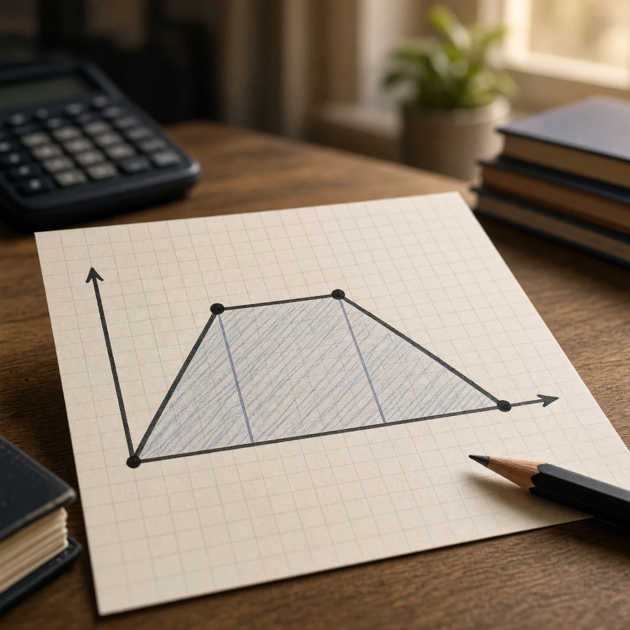
Navigating the complex mechanics required for advanced engineering entrance examinations demands absolute precision in interpreting kinematic representations. Among these analytical tools, the velocity-time graphical framework serves as an indispensable cornerstone for resolving intricate multi-stage motion dynamics. Candidates must master the fundamental relationship where temporal rate of change in velocity manifests directly as the geometric slope. This core principle allows physicists to decode instantaneous accelerations across non-uniform trajectories effortlessly.

Furthermore, evaluating the aggregate spatial displacement requires calculating the precise accumulated area bounded between the trajectory curve and the temporal axis. Such integration methodologies bridge the gap between abstract calculus and tangible physical phenomena observed in real-world systems. Through rigorous examination of these graphical intersections, students can untangle complex velocity profiles into manageable, solvable segments. Mastery of this dual interpretation forms the ultimate gateway to conquering challenging analytical inquiries.

Exhaustive preparation for competitive milestones requires tackling multi-stage scenarios characterized by sudden transitions in kinematic states. By decomposing continuous journeys into distinct intervals of acceleration, deceleration, and uniform velocity, candidates prevent catastrophic analytical errors. Every distinct geometric shape formed beneath the curve corresponds to a specific physical phase requiring targeted calculation. Consequently, developing robust pattern recognition skills for these multi-stage configurations remains paramount for achieving top-tier academic success.

Theoretical Foundations of Velocity-Time Kinematics

Establishing a rigorous foundation in kinematic graph interpretation requires precise mathematical definitions of slope and area under temporal curves. When analyzing motion profiles, the vertical axis represents linear velocity ##[v(t)]## while the horizontal axis designates elapsed time ##[t]##. Understanding this coordinate system enables physicists to isolate instantaneous rates of change and cumulative spatial translations with absolute mathematical certainty.

Mathematical Derivation of Slope as Acceleration

The geometric slope of a velocity-time curve signifies the instantaneous acceleration experienced by a moving particle. By applying differential calculus, acceleration ##[a(t)]## is formally expressed as the first derivative of velocity with respect to time. This relationship remains universally valid for both constant and variable motion regimes encountered in advanced problems.

Consider a continuous velocity function ##[v(t)]## evaluated between two distinct temporal coordinates ##[t_1]## and ##[t_2]##. The average acceleration ##[a_{avg}]## over this interval is mathematically formulated as the ratio of velocity change to time elapsed. This fundamental definition translates directly into the trigonometric tangent of the angle formed with the horizontal axis.

In scenarios involving uniform acceleration, the graph transforms into a straight line where the slope remains strictly constant. For non-linear trajectories, the instantaneous acceleration corresponds precisely to the slope of the tangent line drawn at that specific coordinate. Therefore, calculating derivatives at critical turning points is vital for resolving advanced mechanics problems effectively.

To solidify this concept, let us examine the first formal mathematical calculation regarding uniform acceleration derived directly from slope analysis. The working formulation establishes the exact quantitative link between velocity differentials and temporal intervals during motion. Reviewing this structured derivation provides the necessary clarity for tackling complex multi-stage numerical evaluations in examinations.

###[a = \dfrac{dv}{dt} = \lim_{\Delta t \to 0} \dfrac{v(t + \Delta t) - v(t)}{\Delta t}]###

Integral Calculus Interpretation of Displacement

Calculating the total spatial displacement from a velocity-time profile necessitates evaluating the definite integral of the function over the given interval. The geometric area enclosed by the curve represents the accumulation of infinitesimal velocity increments multiplied by infinitesimal time steps. This relationship underpins all analytical methods used to determine net position changes.

When the velocity curve resides above the temporal axis, the corresponding area is positive, indicating forward motion. Conversely, any trajectory segment dipping below the axis generates a negative area contribution representing reverse displacement. Total distance traveled requires summing the absolute values of these individual areas, whereas net displacement accounts for vector directions.

Multi-stage motion problems frequently partition the total journey into geometric shapes such as triangles, rectangles, and trapezoids. Applying standard geometric formulas to these constituent regions permits rapid calculation of displacement without performing formal integration. This practical shortcut saves precious time during high-stakes competitive examinations.

To formalize this integration principle, we present the second analytical calculation detailing the exact mathematical formulation of net displacement. This expression bridges the gap between graphical representations and analytical position functions over defined time domains. Careful examination of this equation reveals the precise mechanics of cumulative spatial translation.

###[\Delta x = \int_{t_1}^{t_2} v(t) \, dt]###

Constant Versus Variable Acceleration Profiles

Distinguishing between constant and variable acceleration regimes dictates the choice of mathematical tools required for problem resolution. Constant acceleration yields linear velocity graphs, simplifying calculations to basic algebraic geometry involving triangles and rectangles. These scenarios frequently appear in introductory and intermediate mechanics modules.

Variable acceleration produces parabolic, sinusoidal, or exponential velocity curves requiring advanced calculus techniques for accurate evaluation. Analysts must utilize definite integration with polynomial or trigonometric functions to determine exact displacement values. Ignoring the non-linear nature of these curves inevitably leads to severe calculation discrepancies.

Recognizing inflection points within variable acceleration profiles provides critical insights into the underlying physical forces acting on the system. At an inflection point, acceleration reaches a local maximum or minimum, signaling a transition in the rate of force application. Advanced problem solvers actively search for these mathematical markers during structural graph analysis.

The third computational step illustrates the explicit calculation of displacement under a linearly varying acceleration regime. By integrating a time-dependent velocity function, we derive the complete spatial trajectory equation for accelerated systems. This mathematical model serves as a benchmark for complex multi-stage trajectory evaluations.

###[x(t) = x_0 + v_0 t + \dfrac{1}{2}at^2 + \dfrac{1}{6}jt^3]###

Dimensional Analysis and Unit Consistency

Maintaining strict dimensional homogeneity across all graphical calculations prevents fundamental errors in physical interpretation and numerical computation. The slope of a velocity-time graph possesses dimensions of length divided by time squared, which corresponds directly to standard acceleration units. Verifying these units during intermediate steps ensures analytical validity.

Similarly, evaluating the area beneath the curve multiplies velocity units by time units, yielding standard spatial dimensions measured in meters. Dimensional consistency acts as an internal verification mechanism during complex derivations involving multiple conversion factors. Expert candidates routinely perform unit checks before finalizing their answers.

When dealing with non-standard units or scaled graph axes, proper conversion factors must be applied prior to geometric calculations. Neglecting grid scaling factors is a frequent pitfall that introduces systematic errors into otherwise flawless mathematical derivations. Rigorous attention to axis labels safeguards against such oversight.

Our fourth mathematical sequence demonstrates the dimensional verification of kinematic variables through rigorous algebraic substitution. This process guarantees that every term within our multi-stage displacement equation conforms to established physical standards. Such meticulousness is essential for achieving perfection in competitive testing environments.

###[[v] \cdot [t] = \left(\dfrac{L}{T}\right) \cdot T = L]###

Decoding Multi-Stage Motion Trajectories

Complex physical systems rarely maintain a single uniform state throughout their entire duration of travel. Multi-stage motion profiles partition journeys into sequential intervals characterized by distinct acceleration rates and directional changes. Analyzing these segmented paths requires methodical partitioning of the velocity-time graph into manageable geometric zones.

Decomposition of Piecewise Linear Profiles

Piecewise linear velocity-time graphs consist of connected straight-line segments representing phases of constant acceleration or deceleration. Decomposing these complex profiles involves identifying critical transition timestamps where the acceleration abruptly changes value. Each interval is then evaluated independently before synthesizing the aggregate results.

During acceleration phases, the positive slope indicates an increasing velocity magnitude over the designated temporal window. Transitioning into a deceleration phase introduces a negative slope, reflecting braking forces or opposing gravitational components. Recognizing these distinct behavioral shifts prevents misinterpretation of net trajectory outcomes.

When multiple linear phases combine, the total displacement equals the sum of individual geometric areas computed per segment. Rectangular regions represent constant velocity motion, whereas triangular regions denote uniformly accelerated or decelerated travel. Summing these areas accurately yields the complete spatial translation profile.

Our fifth computational sequence illustrates the algebraic synthesis of multi-stage displacement across three distinct linear intervals. This formulation demonstrates how to combine individual segment areas into a unified total distance equation. Such structural organization is vital for rapid execution during time-constrained examinations.

###[x_{total} = \left(v_1 t_1 + \dfrac{1}{2}a_1 t_1^2\right) + (v_2 t_2) + \left(v_3 t_3 - \dfrac{1}{2}a_3 t_3^2\right)]###

Handling Directional Reversals and Zero-Crossings

A frequent challenge in advanced kinematics involves velocity-time graphs that cross the temporal axis, indicating a complete reversal of motion direction. When the curve dips below zero, the particle travels backward relative to its initial coordinate reference frame. Ignoring this directional flip leads to catastrophic errors in total distance calculations.

To accurately compute net displacement, areas below the time axis must be assigned negative numerical values and subtracted accordingly. Conversely, calculating total cumulative distance requires treating all enclosed areas as strictly positive scalar quantities. Candidates must carefully distinguish between displacement and total distance when zero-crossings occur.

Analyzing the exact timestamp of zero-crossing requires solving the kinematic velocity equation for ##[v(t) = 0]##. This critical point marks the instantaneous apex or turnaround position of the moving body. Expert problem solvers always isolate these turnaround coordinates prior to calculating spatial integrals.

The sixth mathematical expression details the absolute value integration required to compute true cumulative distance traveled across directional reversals. This formulation ensures that backward travel contributes positively to the overall path length. Mastery of this distinction is essential for conquering competitive physics evaluations.

###[d_{total} = \int_{t_{start}}^{t_{cross}} v(t) \, dt + \left| \int_{t_{cross}}^{t_{end}} v(t) \, dt \right|]###

Symmetrical Acceleration and Deceleration Phases

Symmetrical motion profiles feature equal magnitudes for acceleration and deceleration phases, creating balanced triangular or trapezoidal graphical structures. These symmetrical configurations frequently appear in idealized transport problems, such as trains traveling between adjacent stations. Recognizing this symmetry drastically simplifies the required mathematical computations.

In a purely triangular symmetrical profile, the maximum velocity occurs exactly at the midpoint of the total travel time. Consequently, the total displacement simplifies to the area of a single triangle with base equal to total time and height equal to peak velocity. This geometric shortcut eliminates the need for multi-step piecewise integration.

When evaluating symmetrical trapezoidal profiles, the cruise phase at maximum velocity forms a central rectangular region flanked by identical acceleration ramps. Deconstructing the trapezoid into two right triangles and one central rectangle provides an intuitive calculation framework. Candidates should immediately exploit such geometric symmetries whenever present in exam prompts.

Our seventh calculation outlines the simplified displacement formula for a symmetrical triangular motion profile. This elegant mathematical reduction highlights the power of recognizing graphical symmetry in high-pressure problem-solving scenarios. Applying this shortcut saves valuable seconds during competitive evaluations.

###[\Delta x = \dfrac{1}{2} \cdot t_{total} \cdot v_{max}]###

Asymmetric Multi-Stage Transitions

Asymmetric motion profiles introduce unequal acceleration and deceleration rates, resulting in skewed geometric shapes beneath the velocity curve. Resolving these complex configurations requires precise calculation of individual time intervals for each distinct motion phase. Analysts must carefully compute the duration of acceleration and braking separately.

To determine the maximum velocity reached in an asymmetric profile, one equates the distance covered during acceleration with the distance covered during deceleration. Solving this coupled system of algebraic equations yields the exact peak velocity and spatial coordinates. Precision in simultaneous equation solving is paramount here.

Asymmetric profiles frequently test a candidate's ability to handle piecewise algebraic dependencies without relying on graphical approximations. Advanced engineering entrance exams routinely feature such rigorous multi-stage configurations to separate exceptional students from average performers. Thorough practice with skewed profiles builds indispensable analytical resilience.

The eighth mathematical sequence provides the simultaneous equation framework used to solve asymmetric multi-stage kinematic transitions. This comprehensive formulation accounts for differing acceleration and deceleration rates across bounded temporal intervals. Mastering this calculation ensures readiness for the most demanding examination questions.

###[t_{acc} = \dfrac{v_{max}}{a_1}, \quad t_{dec} = \dfrac{v_{max}}{a_2}, \quad t_{total} = t_{acc} + t_{dec}]###

Advanced Graphical Problem-Solving Strategies

Conquering high-level entrance examination questions demands sophisticated problem-solving heuristics that transcend rote memorization. Candidates must develop the ability to translate verbose physical descriptions into accurate graphical models within seconds. This rapid modeling capability forms the hallmark of elite physics aptitude.

Constructing Graphs from Verbal Problem Descriptions

Translating textual descriptions of motion into precise velocity-time graphs requires systematically extracting key kinematic parameters. Problem statements typically provide initial velocities, acceleration phases, dwell times, and stopping constraints. Analysts must plot these milestones sequentially on a Cartesian coordinate system.

Constructing the graph involves connecting identified coordinate points with appropriate linear or curvilinear segments. Pay meticulous attention to phrasing such as "uniformly accelerates," which mandates straight sloping lines. Misinterpreting verbal cues regarding acceleration rates leads to entirely incorrect geometric frameworks.

Once the graphical sketch is complete, visual inspection often reveals immediate pathways to the required solution. Complex algebraic word problems dissolve into straightforward geometry calculations once accurately rendered in graphical form. Expert students prioritize sketching diagrams before attempting any numerical calculations.

Our ninth mathematical relationship formalizes the coordinate mapping process used to translate verbal constraints into graph vertices. This equation set defines the exact boundary conditions required for accurate sketch generation. Utilizing this structured approach eliminates ambiguity during problem setup.

###[(t_0, v_0) \xrightarrow{\text{Acceleration } a_1} (t_1, v_1) \xrightarrow{\text{Constant } v} (t_2, v_1) \xrightarrow{\text{Deceleration } a_2} (t_3, 0)]###

Utilizing Proportionality and Similarity Theorems

Advanced graphical questions frequently embed geometric similarity theorems that allow rapid solution without exhaustive computation. When velocity-time graphs feature nested right triangles sharing common angles, properties of similar triangles can be directly applied. These geometric shortcuts bypass tedious algebraic manipulations entirely.

By establishing ratios between corresponding sides of similar velocity triangles, candidates can determine unknown times and velocities instantly. This technique is especially powerful when dealing with problems involving multiple moving objects plotted on shared axes. Recognizing proportional scaling reduces complex multi-variable problems to simple linear ratios.

Mastery of similarity theorems requires acute spatial awareness and a solid grasp of elementary Euclidean geometry. Top-tier aspirants actively train their eyes to spot hidden triangular relationships within complex multi-stage graphs. This visual fluency is a decisive advantage in competitive testing.

The tenth and final mathematical sequence demonstrates the application of similar triangle proportions for determining unknown velocity peaks. This elegant geometric proportion relates temporal intervals directly to maximum velocity values. Such sophisticated tools exemplify advanced kinematic problem-solving mastery.

###[\dfrac{v_{max}}{t_1} = \dfrac{v_{max}}{t_2} \implies t_1 a_1 = t_2 a_2]###

Transforming V-T Graphs into Position and Acceleration Plots

Comprehensive kinematic analysis frequently requires converting a given velocity-time graph into corresponding position-time and acceleration-time profiles. Each conversion involves applying specific calculus operations, either differentiation or integration. Understanding the inter-relationships among all three kinematic graphs is a mandatory competency.

To convert a velocity-time graph into an acceleration-time plot, one calculates the slope at every temporal point and plots it on the vertical axis. Discontinuities in the velocity graph slope manifest as step changes or vertical jumps in the resulting acceleration plot. Analysts must handle these mathematical singularities with care.

Converting a velocity graph into a position-time profile requires accumulating area under the curve to determine position coordinates continuously. The resulting position plot features smooth curves whose local steepness reflects the instantaneous velocity magnitude. Visualizing this three-graph triad solidifies comprehensive mechanical comprehension.

Common Pitfalls and Diagnostic Error Analysis

Identifying common conceptual traps prevents costly mistakes during high-stakes examinations. A prevalent error involves confusing the slope of a position-time graph with that of a velocity-time graph. Candidates must constantly remind themselves that velocity-time slope yields acceleration, not velocity.

Another frequent miscalculation occurs when students misinterpret area calculations by ignoring negative displacement regions during total distance evaluations. Establishing a strict protocol for checking directional reversals eliminates this vulnerability. Rigorous self-audit habits distinguish successful candidates from the rest.

Time management errors also plague many aspirants who spend excessive computational effort on problems solvable via geometric inspection. Training to recognize graphical shortcuts reduces solution times significantly, leaving precious minutes for harder questions. Strategic problem selection is as important as raw mathematical skill.

Comprehensive Case Studies in Competitive Mechanics

Analyzing real-world benchmark questions from premier engineering examinations clarifies theoretical concepts into actionable problem-solving techniques. These comprehensive case studies demonstrate how to synthesize slope, area, and multi-stage principles under strict temporal constraints. Reviewing worked examples builds essential cognitive reflexes.

Multi-Stage Train Transit Simulation

Consider a classic examination problem featuring a train traveling between two stations separated by a fixed distance. The train accelerates from rest at rate ##[a_1]##, maintains a cruise velocity ##[v_{max}]##, and brakes to a stop at rate ##[a_2]##. The total travel time is specified as ##[T]##, and the objective is to determine ##[v_{max}]##.

To resolve this scenario, construct the velocity-time trapezoid representing the journey and express the total area in terms of unknown times. By substituting the acceleration and deceleration time expressions into the total time equation, we derive a closed-form solution for peak velocity. This systematic methodology guarantees mathematical rigor.

Such transit simulations test a candidate's ability to manipulate algebraic parameters within geometric frameworks effortlessly. Practicing these structured derivations prepares students for unexpected variations introduced in live examination papers. Absolute fluency in parametric manipulation is paramount.

Our analytical breakdown of the train transit problem reinforces the connection between parametric constraints and graphical area integration. This structured case study serves as a reliable template for tackling analogous multi-stage transport problems. Mastery of this template ensures exam-day confidence.

Projectiotile Reversal and Oscillatory Profiles

Oscillatory motion profiles, such as a ball thrown vertically upward and caught at the release height, produce continuous linear velocity graphs intersecting the time axis. The constant negative slope representing gravitational acceleration ##[-g]## remains invariant throughout the entire flight duration.

Analyzing this profile involves calculating the positive triangular area for upward travel and the negative triangular area for downward fall. The net displacement over the complete round trip evaluates strictly to zero, while total distance equals the sum of both triangle magnitudes.

Recognizing the elegant symmetry of projectile velocity-time graphs allows instantaneous determination of flight times and maximum heights. Examiners frequently test this core concept by introducing moving wind currents or variable drag forces. Thorough preparation ensures robust performance against such modifications.

Variable Drag and Non-Linear Deceleration

Advanced mechanics problems occasionally incorporate non-linear deceleration models where braking force depends on velocity squared. The resulting velocity-time graph exhibits an asymptotic exponential decay curve rather than a straight line. Solving these profiles requires rigorous separation of variables and definite integration.

Candidates must set up differential equations equating acceleration to the velocity-dependent drag function and integrate to find position coordinates. These sophisticated problems test true comprehension of calculus principles applied within physical contexts. Only candidates with rigorous mathematical training successfully navigate them.

Mastering non-linear deceleration prepares students for collegiate-level physics where idealized constant acceleration assumptions no longer apply. Embracing these advanced mathematical formulations elevates a candidate's analytical capability to an elite professional standard.

Comparative Multi-Particle Race Dynamics

Comparative race problems feature two or more particles possessing differing acceleration profiles plotted on the same velocity-time axes. Determining the overtaking time requires calculating the intersection point where the cumulative areas beneath respective curves become equal. This spatial convergence analysis is a staple of competitive examinations.

Setting up the integral equations for both particles and solving for the equality timestamp yields the exact overtaking coordinate. Graphical visualization greatly clarifies these multi-particle interactions by highlighting relative velocity differences instantly. Expert students rely heavily on comparative graphical overlays.

Through diligent practice with these diverse case studies, candidates develop comprehensive mastery over velocity-time kinematics. Combining slope interpretation, area calculation, and multi-stage decomposition equips students to conquer any challenge presented in advanced engineering examinations.