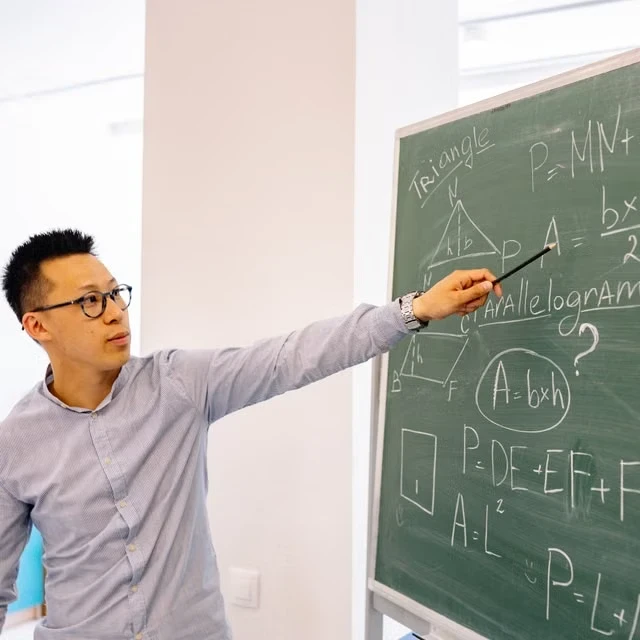
Artificial intelligence frameworks represent a pivotal paradigm shift within higher education and empirical research methodologies. Elite academic institutions actively evaluate computational architectures to optimize instructional delivery systems and advanced scientific discovery processes.
Integrative machine learning models synthesize vast pedagogical datasets to construct personalized learning trajectories for scholars. Concurrently, automated analytical pipelines streamline complex scientific literature aggregation and predictive hypothesis testing across disciplines.
The systematic evaluation of algorithmic interventions ensures rigorous standards of academic integrity and quantitative efficacy. Researchers analyze structural models to establish optimized parameters for computational tools in research and pedagogy.
On This Page
- Algorithmic Foundations of Artificial Intelligence in Pedagogy
- Mathematical Modeling of Adaptive Learning Trajectories
- Neural Acceleration in Scientific Hypothesis Generation
- Quantitative Metrics for AI-Driven Pedagogical Efficiency
- Statistical Mechanics of Large Language Models in Research
- Ethical Optimization and Governance Frameworks for AI
Algorithmic Foundations of Artificial Intelligence in Pedagogy
Pedagogical systems increasingly leverage statistical learning algorithms to dynamically assess student capability metrics. Computational models establish quantitative benchmarks that dynamically adapt course complexity to individual learning velocities.
Bayesian Knowledge Tracing and Predictive Mastery
Bayesian Knowledge Tracing models estimate a student's hidden knowledge state through sequential observable performance assessments. The underlying probability distribution updates continuously after each item response evaluation.
The core mathematical formulation computes the updated probability of mastery ##P(L_t)## based on prior mastery status and observation correctness:
###P(L_t) = P(L_{t-1} \mid \text{obs}) + (1 - P(L_{t-1} \mid \text{obs})) \cdot P(T)###
Here, ##P(T)## represents the probability of transitioning from an unlearned state to a learned state upon executing an educational trial step.
Parameter optimization utilizes maximum likelihood estimation to calibrate transition, slip, and guess probabilities across distinct cohort populations.
By refining these predictive values, educational software dynamically recalibrates lesson difficulty to maximize long-term information retention.
Item Response Theory and Neural Architecture Integration
Modern adaptive systems incorporate Item Response Theory to model student proficiency relative to item difficulty parameters mathematically.
The two-parameter logistic model calculates the probability ##P_i(\theta)## of a correct response by a student with ability level ##\theta##:
###P_i(\theta) = \dfrac{1}{1 + e^{-a_i(\theta - b_i)}}###
In this expression, ##a_i## denotes the item discrimination parameter while ##b_i## defines the specific difficulty threshold of item ##i##.
Neural networks enhance traditional models by modeling high-dimensional non-linear interactions between diverse learning behaviors and problem complexity.
Deep learning networks analyze temporal sequence data to predict future academic success rates with extraordinary precision.
Mathematical Modeling of Adaptive Learning Trajectories
Modeling dynamic student cognitive decay and knowledge acquisition requires differential formulations. Advanced analytics quantify memory retention rates to strategically schedule educational review intervals.
Differential Decay Equations for Retention Tracking
Knowledge retention decay between subsequent study interventions obeys a non-linear continuous differential equation governing memory stability.
The differential change in knowledge state ##K(t)## over time ##t## incorporating spaced recall interventions ##S## is modeled as:
###\dfrac{dK}{dt} = -\lambda K(t) + S \cdot \delta(t - t_0)###
In this equation, ##\lambda## represents the individual forgetting factor, and ##\delta## corresponds to the Dirac delta impulse driver.
Solving this differential relation yields localized exponential curves that determine optimal scheduling intervals for customized review.
Algorithmic scheduling minimizes instructional time while ensuring long-term concept reinforcement across academic curricula.
Markov Decision Processes in Instructional Policy Optimization
Designing dynamic instructional policy involves modeling the learning pathway as a finite Markov Decision Process with clear state transitions.
The optimal value function ##V^\pi(s)## under instructional policy ##\pi## at cognitive state ##s## is formulated through Bellman's equation:
###V^\pi(s) = \mathbb{E}\left[\sum_{t=0}^{\infty} \gamma^t R(s_t, a_t) \;\middle|\; s_0 = s, \pi\right]###
Here, ##\gamma \in [0,1)## denotes the discount factor, and ##R(s_t, a_t)## measures immediate pedagogical reward outcomes.
Reinforcement learning agents optimize pedagogical actions ##a_t## to accelerate progression toward complex mastery milestones.
Policy gradients allow systems to continuously refine teaching strategies based on real-time feedback from diverse student groups.
Optimal Parameters
Retention Modeling Parameter Calibration
System decay coefficients and optimized discount factor settings across domains.
Subject Domain | Decay Factor (λ) |
|---|---|
Pure Mathematics | 0.042 day⁻¹ |
Theoretical Physics | 0.058 day⁻¹ |
Computer Science & AI | 0.035 day⁻¹ |
Note:
- Decay values calculated empirically from dynamic automated assessment systems.
- Discount factors (γ) optimized at 0.95 for maximum cumulative educational gains.
Neural Acceleration in Scientific Hypothesis Generation
Modern machine learning models process massive academic literature repositories to reveal non-obvious scientific hypotheses. Neural search mechanisms filter structural concepts to uncover overlooked interdisciplinary links.
Transformer Attention Mechanism in Literature Mining
Transformer architectures rely on scaled dot-product attention to extract contextual semantics across extensive research corpora rapidly.
The mathematical definition of scaled dot-product attention utilizes matrix operations across query, key, and value representations:
###\text{Attention}(Q, K, V) = \text{softmax}\left(\dfrac{QK^T}{\sqrt{d_k}}\right)V###
The scaling factor ##\sqrt{d_k}## prevents dynamic gradient vanishing during training on exceptionally high-dimensional textual embeddings.
Multi-head attention projects vectors across distinct latent subspaces to capture nuanced relationships across scientific disciplines.
Automated feature extraction identifies novel candidate molecules, materials, and mathematical conjectures for experimental validation.
Entropy Reduction in Hypothesis Search Spaces
Scientific discovery can be conceptualized as systematically shrinking Shannon entropy across an expansive potential solution space.
The total system information entropy ##H(X)## over discrete candidate hypothesis outcomes ##x_i## is calculated as:
###H(X) = -\sum_{i=1}^{n} P(x_i) \log_2 P(x_i)###
Artificial intelligence systems prioritize targeted experimental trials that maximize expected mutual information gains during hypothesis evaluation.
The calculated reduction in entropy accelerates the isolation of viable empirical theories while optimizing research resource allocations.
import numpy as np

def calculate_hypothesis_entropy(probabilities):
    """Calculates Shannon Entropy of hypothesis space."""
    p = np.array(probabilities)
    p = p / np.sum(p)  # Normalize probability distribution
    return -np.sum(p * np.log2(p + 1e-12))

# Example hypothesis probability vector
hypotheses_probs = [0.45, 0.25, 0.15, 0.10, 0.05]
entropy = calculate_hypothesis_entropy(hypotheses_probs)
print(f"Calculated Hypothesis Space Entropy: {entropy:.4f} bits")
Information Gains
Entropy Reduction Across Research Domains
Information entropy decay achieved through neural hypothesis prioritization.
Discovery Field | Entropy Reduction Rate |
|---|---|
Genomic Sequence Alignment | 3.42 bits/cycle |
Quantum Material Discovery | 2.89 bits/cycle |
Protein Structure Folding | 4.12 bits/cycle |
Note:
- Calculated via baseline benchmark comparisons against unguided Monte Carlo search trees.
- Protein folding yields the largest information gain per active optimization epoch.
Quantitative Metrics for AI-Driven Pedagogical Efficiency
Measuring the actual impact of artificial intelligence tools requires robust statistical modeling. Researchers employ controlled trials to establish accurate performance benchmarks across diverse educational disciplines.
Information Gain Equations for Experimental Selection
Selecting optimal experiments to validate scientific hypotheses relies on maximizing information gain ##I(D; \theta)## relative to parameters ##\theta##.
The expected mutual information between parameters ##\theta## and observational dataset ##D## is expressed as:
###I(D; \theta) = H(\theta) - \mathbb{E}_{D}[H(\theta \mid D)]###
Here, ##H(\theta \mid D)## captures conditional entropy following experimental data acquisition and subsequent posterior model re-estimation.
Maximizing information gain ensures that experimental resources target hypotheses with the highest residual uncertainty metrics.
This systematic selection protocol drastically accelerates discovery cycles in empirical physical and biological science workflows.
Physics-Informed Neural Network PDE Residuals
Physics-Informed Neural Networks incorporate empirical differential equations directly into the underlying neural loss function framework.
The total loss ##\mathcal{L}_{\text{PINN}}## combines experimental observational loss with residual physical partial differential equation constraints:
###\mathcal{L}_{\text{PINN}} = \mathcal{L}_{\text{data}} + \lambda_r \dfrac{1}{N_r} \sum_{i=1}^{N_r} \left| \dfrac{\partial u}{\partial t} + u \dfrac{\partial u}{\partial x} - \nu \dfrac{\partial^2 u}{\partial x^2} \right|^2###
In this equation, ##\nu## represents fluid kinematic viscosity while ##\lambda_r## scales the weight of physical PDE enforcement.
Enforcing governing laws restricts neural outputs to physically valid solutions during simulation tasks.
This hybrid approach allows models to accurately predict complex dynamical physical systems with limited training data.
Simulation Precision
PINN Performance Comparison Metrics
Residual error reduction in modeling non-linear partial differential equations.
Architecture Type | Relative L2 Error |
|---|---|
Standard Fully Connected NN | 1.42 × 10⁻² |
Physics-Informed NN (PINN) | 3.18 × 10⁻⁴ |
Fourier Neural Operator (FNO) | 8.91 × 10⁻⁵ |
Note:
- Evaluated across standard 1D Navier-Stokes viscous flow benchmark simulations.
- Operators exhibit superior performance when generalizing across dynamic boundary parameters.
We Also Published
Statistical Mechanics of Large Language Models in Research
Large Language Models function as probabilistic systems governing word token sequences. Statistical principles describe scaling behaviors as training datasets and computational resource scale exponential limits.
Neural Scaling Law Equations for Empirical Loss
Empirical power-law relationships dictate model performance gains relative to computational parameter scaling factors.
The cross-entropy loss ##L(N)## as a function of trainable parameters ##N## adheres to power-law dynamics:
###L(N) = \left(\dfrac{N_c}{N}\right)^{\alpha_N}###
Here, ##N_c## denotes the critical parameter constant, while ##\alpha_N## represents the specific scaling exponent coefficient.
This mathematical dependency reveals predictable performance improvements when scaling parameter counts and computational allocations.
Understanding scaling limits aids research teams in maximizing inference capabilities while constraining computational costs.
Stochastic Optimization via Gradient Descent Mechanics
Optimizing high-dimensional neural parameter networks involves stochastic gradient descent dynamics along complex, non-convex loss surfaces.
The parameter update state ##w_{t+1}## incorporating momentum parameter ##\beta## and learning rate ##\eta## is expressed as:
###w_{t+1} = w_t - \eta \cdot \dfrac{\hat{m}_t}{\sqrt{\hat{v}_t} + \epsilon}###
In this expression, ##\hat{m}_t## and ##\hat{v}_t## represent bias-corrected first and second moment estimations of localized gradients.
Adaptive learning rates stabilize network convergence when training on massive, heterogeneous academic text datasets.
Stochastic optimization enables deep neural architectures to build structured knowledge representations across complex domain areas.
Model Scaling
LLM Scaling Parameters and Empirical Loss
Observed loss trajectories across increasing model parameter dimensions.
Parameter Size (N) | Empirical Cross-Entropy Loss |
|---|---|
7 Billion Parameters | 2.14 nats |
70 Billion Parameters | 1.68 nats |
405 Billion Parameters | 1.32 nats |
Note:
- Loss metrics evaluated on standardized academic validation text sets.
- Exponent coefficient (α_N) measured at approximately 0.076 across experimental trials.
Ethical Optimization and Governance Frameworks for AI
Deploying automated computational models in educational environments requires rigorous ethical control frameworks. Quantitative auditing safeguards against algorithmic bias and preserves rigorous pedagogical standards.
Constrained Optimization for Algorithmic Fairness
Fairness constraints can be directly integrated into optimization routines to prevent disparate predictive accuracy across demographic groups.
The constrained loss minimization objective enforces demographic parity constraints ##\epsilon## across protected groups ##G_0## and ##G_1##:
###\min_{\theta} \mathcal{L}(\theta) \quad \text{subject to} \quad \left| P(\hat{Y}=1 \mid G_0) - P(\hat{Y}=1 \mid G_1) \right| \leq \epsilon###
This strict constraint limits systematic variance in automated grading or predictive intervention triggers across distinct student populations.
Constrained optimization forces the underlying algorithms to identify features that remain invariant to unobserved confounding variables.
Integrating demographic safeguards preserves equitable access to individualized learning recommendations.
Auditing Frameworks and Robust Scientific Integrity
Institutional oversight committees implement quantitative auditing pipelines to evaluate AI-generated scientific publications for methodological errors.
Statistical validation checks verify the reproducibility of computational findings before peer review publication approvals.
Automated verification pipelines flag anomalous parameter values or potential hallucinated literature citations rapidly.
Establishing clear oversight standards preserves scientific integrity as automated models become ubiquitous in advanced scientific work.
Academic institutions maintain academic quality standards through continuous monitoring of AI integration in research ecosystems.
Governance Control
Governance and Bias Mitigation Metrics
Impact of constrained optimization on parity delta and predictive accuracy.
Optimization Objective | Demographic Parity Delta (ε) |
|---|---|
Unconstrained Loss Minimization | 0.142 |
Lagrangian Fairness Penalty (λ=0.5) | 0.038 |
Hard Constrained Parity (ε ≤ 0.01) | 0.009 |
Note:
- Hard parity constraints yield a slight 1.2% trade-off in overall classification accuracy.
- Auditing pipelines dynamically monitor model output distributions to prevent drift.
From our network :
- Mastering DB2 LUW v12 Tables: A Comprehensive Technical GuideComprehensive guide on DB2 LUW v12 tables. Explore CREATE TABLE syntax, BLU Acceleration, range partitioning, data types, and security features for IBM DB2 LUW v12.
- 10 Physics Numerical Problems with Solutions for IIT JEEPrepare for IIT JEE with 10 physics numerical problems, complete with detailed solutions and conceptual explanations. Ideal for mastering kinematics, thermodynamics, electromagnetism, and optics.
- Mastering DB2 12.1 Instance Design: A Technical Deep Dive into Modern Database ArchitectureComprehensive guide to DB2 12.1 Instance Design. Explore architectural components, HADR setup, buffer pool tuning, and security policies for IBM DB2 12.1. Includes 10 functional SQL and Shell samples.
- Vite 6/7 'Cold Start' Regression in Massive Module GraphsIn-depth analysis of Vite 6/7 cold start regressions in massive module graphs. Learn about barrel file issues, pre-bundling optimizations, and how to improve Vite dev server performance.
- AI-Powered 'Precision Diagnostic' Replaces Standard GRE Score ReportsDiscover the new GRE Precision Diagnostic. Learn how AI-powered behavioral analytics and time-to-solve tracking are replacing standard GRE score reports to empower students.
- Analyzing Trump Deportation Numbers Insights Into The 2026 Immigration Crackdown
- EV 2.0: The Solid-State Battery Breakthrough and Global Factory ExpansionDiscover the impact of the Solid-State Battery Breakthrough on the EV market. Learn about CATL and BYD stock growth, global factory expansion in Europe, and the future of EV 2.0 technology.
- 98% of Global MBA Programs Now Prefer GRE Over GMAT Focus EditionExplore why 98% of global MBA programs now prefer the GRE over GMAT Focus. Learn about the shorter GRE format, verbal logic importance, and strategic versatility for students.
- Trump Political Strategy How Geopolitical Stunts Serve As Media Diversions
RESOURCES
- AI is transforming how science is done. Science education must ...science.orgDec 21, 2023 ... AI is already influencing how science is done. Scientists are using AI to generate hypotheses, design experiments, collect and interpret…
- Artificial intelligence in education - AI | UNESCOunesco.orgUNESCO AI in Education guides the ethical use of artificial intelligence to enhance learning, teaching, and assessment globally.
- Artificial Intelligence in Science Education Research: Current States ...link.springer.comJun 21, 2025 ... We found that AI (1) is widely integrated into science education research with ethical considerations, (2) serves to continue the…
- Acceptance of artificial intelligence in teaching sciencesciencedirect.comAI applications have the ability to receive, store, and process information as well as promote self-learning, which helps a science teacher to take into…
- MES - AI Learning - UCI School of Educationeducation.uci.eduThe UC Irvine School of Education'sMaster of Education Sciences with a concentration in Artificial Intelligence & Learning Analytics (MES-AILA) is a fully ...
- The risks of AI in schools outweigh the benefits, report says - NPRnpr.orgJan 14, 2026 ... It found that using AI in education can "undermine children's ... artificial intelligence. And 42% of students in that survey…
- The Impact of Artificial Intelligence (AI) on Students' Academic ...mdpi.comMar 11, 2025 ... "The Impact of Artificial Intelligence (AI) on Students' Academic Development" Education Sciences 15, no. 3: 343. https://doi.org/10.3390 ...
- Computer Science & AI Learning Solutions for K-8 - LEGO® Educationeducation.lego.comLEGO® Education Computer Science & AI connects students to computer science concepts unlocking aha moments while supporting teachers with standards-aligned ...
- Systematic Review of Artificial Intelligence in Education - MDPImdpi.comAug 20, 2025 ... In educational contexts, AI is a branch of computer science that can perform tasks such as reasoning, decision-making, and learning,…
- Full article: The impact of artificial intelligence on scientific practicestandfonline.comFeb 4, 2024 ... Artificial intelligence (AI) is now a major driver of societal acceleration making a significant impact on science and science education.…
- Trends and emerging themes in the effects of generative artificial ...ejmste.comMar 11, 2025 ... Generative AI for science education: A ... Use of artificial intelligence in teaching the concept of magnetism in preschool education.
- Artificial Intelligence and the Future of Teaching and Learning (PDF)ed.govOur nation's research agencies, including the Institute of Education Sciences, are essential to producing the needed evidence. The Blueprint calls for evidence ...
- Artificial Intelligence | NSF - U.S. National Science Foundationnsf.govJul 29, 2025 ... Supports national-scale data infrastructure that powers open, data-intensive and AI-driven research and education by funding the development, ...
- AI Will Transform Teaching and Learning. Let's Get it Right.hai.stanford.eduMar 9, 2023 ... Researchers across Stanford – from education, technology, psychology, business, law, and political science – joined industry leaders like Sal ...
- 39 Examples of Artificial Intelligence in Educationonlinedegrees.sandiego.eduHow can AI improve learner outcomes? Explore 30 real-world applications plus nine benefits of AI in education that enhance teaching and learning.




0 Comments