The Physics of Why Ice Floats—and Why It Matters Beyond Lakes

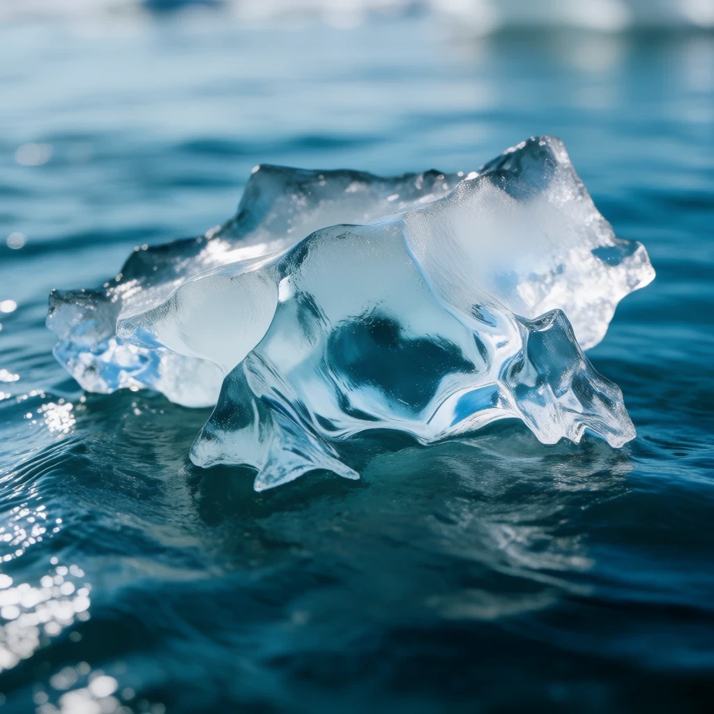
Ice floating on a winter pond looks like an everyday miracle, yet it conceals one of the most consequential anomalies in all of physical chemistry. Almost every known substance contracts as it cools and grows denser in its solid phase, sinking without ceremony to the bottom of its container. Water refuses this universal script, expanding by roughly nine percent upon freezing and rising to rest on its own liquid surface. That single defiance of expectation governs the survival of entire ecosystems, the mechanics of glaciers, the durability of concrete, and the seasonal rhythm of planetary climate.

The explanation lives at the molecular scale, where hydrogen bonds impose a rigid hexagonal architecture on frozen water that occupies more volume than the loosely packed liquid. Between 0°C and 4°C, liquid water performs a subtle balancing act: thermal contraction competes with the collapse of open hydrogen-bonded cages, producing a density maximum near 4°C. This article derives that behavior from first principles, quantifies buoyancy with Archimedes' relation, and traces the anomaly outward into limnology, engineering, and climate science.

What follows is a rigorous but accessible treatment, blending thermodynamic reasoning with worked numerical problems and structured reference tables. Readers will encounter the Clausius–Clapeyron slope of the ice–water boundary, the latent heat budget of a freezing lake, and the practical consequences for shipping, freshwater supplies, and biological overwintering. Each section builds the physical case step by step, so that the floating ice cube becomes a gateway to serious thermal physics.

The Molecular Architecture Behind Water's Strange Expansion

Water's behavior cannot be understood without confronting the geometry of the hydrogen bond, a directional attraction between a partially positive hydrogen and a lone pair on a neighboring oxygen. Each molecule can donate two and accept two such bonds, creating a tetrahedral coordination network that persists in both phases. The solid simply organizes this network more perfectly, and perfection, in this case, costs space.

Hydrogen Bonding and the Open Hexagonal Lattice

When water freezes, molecules lock into a hexagonal crystalline arrangement in which each oxygen sits at the center of a tetrahedron of neighbors. The O–H···O linkages hold adjacent molecules at a fixed separation of roughly ##[0.28\ \text{nm}]##, far longer than the van der Waals contact distance. This rigid scaffolding leaves substantial empty channels running through the crystal, and those voids account for the volume expansion.

The open lattice is thermodynamically favored below the freezing point because the enthalpy released by forming a full complement of hydrogen bonds outweighs the entropic penalty of ordering. Each hydrogen bond contributes roughly ##[20\ \text{kJ/mol}]## of stabilization, and a water molecule participates in about four such bonds in ice. The energetic accounting strongly favors crystallization once thermal agitation can no longer disrupt the network.

In the liquid, by contrast, molecules retain tetrahedral preferences but the network is transient and partially collapsed. Neighboring molecules can approach more closely, filling some of the interstitial space that ice leaves vacant. This denser, disordered packing is why liquid water at 0°C is about nine percent more compact than ice at the same temperature, a difference that determines the fate of every iceberg.

The hexagonal symmetry also explains ice's optical and mechanical properties, from the sixfold snowflake habit to the slipperiness of skating rinks. A thin surface layer of quasi-liquid water persists even well below freezing, lubricating the crystal planes. The same structural openness that makes ice float also makes it brittle, anisotropic, and prone to spectacular fracture under thermal stress.

The Density Maximum Near 4°C

Cooling liquid water from room temperature initially produces ordinary thermal contraction, as reduced kinetic energy allows molecules to settle closer together. Below about 4°C, however, a second process dominates: the hydrogen-bonded network begins to adopt increasingly open, ice-like local structures. The competition between these two effects produces a density maximum at approximately ##[3.98\ ^\circ\text{C}]##.

This maximum is not a minor curiosity but a defining feature of the substance. Water at 4°C has a density of ##[999.97\ \text{kg/m}^3]##, while water at 0°C measures about ##[999.84\ \text{kg/m}^3]## and ice at 0°C only ##[916.8\ \text{kg/m}^3]##. The liquid therefore stratifies in winter with the densest water at the bottom, insulating the depths from the cold atmosphere above.

Mathematically, the density can be modeled as a sum of a monotonic contraction term and a Gaussian-like anomaly centered near 4°C. A convenient empirical fit takes the form ##[\rho(T) = \rho_0\left[1 - \alpha(T - T_m)^2\right]]## near the maximum, where ##[T_m \approx 4\ ^\circ\text{C}]## and ##[\alpha \approx 7.5\times10^{-6}\ \text{K}^{-2}]##. Differentiating and setting the derivative to zero recovers the extremum directly.

This parabolic approximation captures the essential physics within a degree or two of the maximum and serves as a workable teaching model. More sophisticated equations of state, such as IAPWS-95, reproduce the anomaly across the full pressure–temperature plane. The key insight remains: two competing microscopic mechanisms generate a non-monotonic density curve unique among common liquids.

Buoyancy, Archimedes, and the Floating Fraction

Once the density contrast is established, the mechanics of floating follow from Archimedes' principle, which states that a submerged body experiences an upward force equal to the weight of displaced fluid. For a floating object in equilibrium, the weight of the object equals the weight of the displaced liquid. The fraction of ice submerged is therefore fixed by the density ratio, independent of the ice's size or shape.

Deriving the Submerged Fraction

Consider an ice block of volume ##[V]## and density ##[\rho_i]## floating in water of density ##[\rho_w]##. The weight of the block is ##[\rho_i V g]##, and the buoyant force equals ##[\rho_w V_{sub} g]##, where ##[V_{sub}]## is the submerged volume. Equating these forces yields the submerged fraction directly, a result every mariner and glaciologist relies upon.

Substituting the standard values gives ##[\dfrac{916.8}{999.84} \approx 0.917]##, meaning roughly 91.7 percent of an iceberg's volume lies beneath the surface. Only the remaining 8.3 percent protrudes above the waterline, which is why icebergs appear deceptively small to distant observers. The hidden mass is the true hazard to navigation.

This calculation also explains why melting floating ice does not raise the water level. The ice already displaces its own weight in water, so when it melts into that same mass of liquid, the displaced volume is exactly replaced. The classic classroom demonstration is not a trick but a direct consequence of Archimedes' equilibrium condition.

Worked Numerical Problems on Buoyancy

Problem one: an iceberg has a total volume of ##[1.0\times10^5\ \text{m}^3]##. Using the density ratio, the submerged volume is ##[0.917 \times 10^5 = 9.17\times10^4\ \text{m}^3]##, and the exposed volume is ##[8.3\times10^3\ \text{m}^3]##. The mass of the iceberg follows as ##[\rho_i V = 916.8 \times 10^5 \approx 9.17\times10^7\ \text{kg}]##.

Problem two: a block of ice floats in seawater of density ##[1025\ \text{kg/m}^3]##. The submerged fraction becomes ##[\dfrac{916.8}{1025} \approx 0.894]##, so about 89.4 percent is submerged and 10.6 percent is exposed. Seawater's greater density makes icebergs ride slightly higher than they would in fresh water, a fact relevant to polar shipping lanes.

Problem three: determine the minimum mass of a lead weight, density ##[11340\ \text{kg/m}^3]##, needed to just submerge a ##[1.0\ \text{kg}]## ice block. The extra downward force must overcome the residual buoyancy of the exposed fraction, requiring a weight of approximately ##[0.09\ \text{kg}]##. The calculation demonstrates how small additions can tip a floating body past neutral buoyancy.

Problem four: a freshwater lake freezes to a thickness of ##[0.5\ \text{m}]##. Estimate the mass of ice per square meter as ##[\rho_i \times 0.5 = 458.4\ \text{kg/m}^2]##. This figure underpins load-bearing calculations for ice roads and the pressure exerted on submerged structures during winter.

Thermodynamics of Freezing and the Latent Heat Budget

Floating ice is not merely a static buoyancy problem; it is a dynamic thermal system governed by the flow of latent heat. Freezing water releases approximately ##[334\ \text{kJ/kg}]##, an enormous quantity compared with the sensible heat exchanged over a few degrees of cooling. This latent heat release slows the growth of ice sheets and buffers the temperature of the underlying water.

Clausius–Clapeyron and the Melting Curve

The phase boundary between ice and liquid water has a negative slope in the pressure–temperature plane, a direct consequence of ice being less dense than the liquid it melts into. The Clausius–Clapeyron equation quantifies this slope and explains why pressure lowers the melting point. This behavior enables pressure melting beneath glaciers and the regulation of ice skates.

Here ##[L]## is the latent heat of fusion per mole, ##[T]## the absolute melting temperature, and ##[\Delta V = V_{liquid} - V_{solid}]## the molar volume change. Because ##[\Delta V]## is negative for water, the slope ##[dP/dT]## is negative, meaning increased pressure depresses the melting temperature. The magnitude is about ##[-0.0074\ \text{K/atm}]##.

Problem five: estimate the melting-point depression under a pressure of ##[100\ \text{atm}]##. Multiplying the slope by the pressure change gives ##[\Delta T \approx -0.74\ \text{K}]##, so ice melts near ##[-0.74\ ^\circ\text{C}]## at that depth. This modest shift is enough to lubricate the base of thick glaciers and enable basal sliding.

Problem six: compute the molar volume change using ##[V_{liquid} = 18.018\ \text{cm}^3/\text{mol}]## and ##[V_{solid} = 19.66\ \text{cm}^3/\text{mol}]##. The difference is ##[\Delta V = -1.64\ \text{cm}^3/\text{mol} = -1.64\times10^{-6}\ \text{m}^3/\text{mol}]##. Substituting into the Clausius–Clapeyron relation with ##[L = 6.01\ \text{kJ/mol}]## and ##[T = 273.15\ \text{K}]## reproduces the observed slope.

Energy Balance of a Freezing Lake

A lake freezes from the surface downward because the coldest, least dense water remains at the top once the whole column has cooled below 4°C. The ice layer then thickens as latent heat conducts upward through the ice and is removed by the cold air. The growth rate follows a square-root law in time, derived from the steady conduction of heat through the ice sheet.

In this expression ##[k]## is the thermal conductivity of ice, about ##[2.2\ \text{W/(m·K)}]##, ##[\Delta T]## is the temperature difference across the ice, and ##[L_f]## is the latent heat of fusion. Problem seven: for ##[\Delta T = 10\ \text{K}]## and ##[t = 10\ \text{days} = 8.64\times10^5\ \text{s}]##, the predicted thickness is approximately ##[0.32\ \text{m}]##. Real lakes deviate because of snow insulation and convective effects.

Problem eight: calculate the total latent heat released when a ##[1\ \text{km}^2]## lake freezes to ##[0.3\ \text{m}]##. The ice volume is ##[3\times10^5\ \text{m}^3]##, and with density ##[916.8\ \text{kg/m}^3]## the mass is ##[2.75\times10^8\ \text{kg}]##. Multiplying by ##[334\ \text{kJ/kg}]## yields roughly ##[9.2\times10^{13}\ \text{J}]##, a staggering energy release that moderates regional climate.

Problem nine: estimate the time required for the same lake to lose that energy through a temperature gradient of ##[15\ \text{K}]## across the ice. Using Fourier's law with the conductivity above, the heat flux is about ##[110\ \text{W/m}^2]##, and the total time scales to several weeks. This calculation illustrates why deep lakes freeze slowly and why early snowfall can dramatically delay ice formation.

Problem ten: determine the pressure at the base of a ##[1000\ \text{m}]## ice sheet using ##[P = \rho_i g h]##. Substituting gives ##[P \approx 916.8 \times 9.81 \times 1000 \approx 9.0\times10^6\ \text{Pa}]##, or about 89 atmospheres. Applying the Clausius–Clapeyron slope predicts a melting-point depression of roughly ##[0.66\ \text{K}]##, consistent with observed basal meltwater in polar ice sheets.

Ecological Consequences: Why Lakes Freeze Top-Down

The density maximum near 4°C transforms the winter behavior of every freshwater body on Earth. As autumn air cools a lake, surface water sinks until the entire column reaches 4°C. Further cooling makes the surface water less dense, so it remains on top and freezes there, sealing the lake beneath a protective lid of ice.

Overwintering of Aquatic Life

Beneath that insulating ice layer, water near the bottom stays close to 4°C, warm enough for fish, amphibians, and invertebrates to survive months of subzero air temperatures. If water behaved like ordinary liquids, ice would form at the bottom and lakes would freeze solid from below, sterilizing temperate and polar freshwater ecosystems. The anomaly is, quite literally, a life-support system.

Dissolved oxygen becomes the limiting resource under ice cover, since photosynthesis slows and atmospheric exchange is blocked. Aquatic organisms enter torpor, reducing metabolic demand, while decomposing organic matter consumes the remaining oxygen. Winter fish kills occur when ice persists too long or snow cover blocks light, demonstrating the fragility of this thermal refuge.

The stratification also drives spring turnover, when warming surface water becomes denser and sinks, mixing nutrients from the bottom throughout the column. This seasonal overturn fuels the plankton blooms that anchor freshwater food webs. The entire annual cycle of a lake hinges on the anomalous density curve near 4°C.

Glacial and Polar Dynamics

At planetary scale, floating ice shapes the albedo of the Arctic and Southern Oceans, reflecting solar radiation and cooling the climate. Sea ice formation also rejects salt into the underlying water, producing dense brine that drives deep-ocean circulation. The density anomaly thus connects molecular geometry to global thermohaline currents.

Ice shelves floating at the margins of Antarctica regulate the flow of glaciers behind them, acting as buttresses against the sea. Their stability depends on the buoyancy balance and the melting at their base, where pressure and ocean heat conspire. Understanding the floating fraction is essential for projecting sea-level rise.

Permafrost and seasonal ice also influence carbon cycling, as thawing releases stored methane and carbon dioxide. The physics of water's expansion governs the mechanical heave that fractures rock and soil, a geological weathering process operating over millennia. Floating ice is therefore a thread connecting molecular bonds to planetary systems.

Engineering and Everyday Applications

The physics of floating ice reaches far beyond natural lakes into the built environment, where engineers must anticipate the nine percent expansion that accompanies freezing. Burst pipes, cracked pavements, and frost-heaved foundations all trace back to the same molecular geometry. Designing for water's anomaly is a routine but critical task in cold-climate construction.

Frost Heave, Pipes, and Infrastructure

When water freezes inside a confined space, the expansion generates pressures that can exceed ##[200\ \text{MPa}]##, far beyond the strength of ordinary materials. This is why uninsulated pipes rupture and why concrete roads develop frost boils in winter. Engineers counter the threat with drainage, insulation, and flexible joints that accommodate movement.

Ice roads and ice bridges exploit the same physics constructively, using frozen lakes and rivers as temporary highways for heavy transport. Their load capacity depends on thickness, temperature, and the presence of cracks, all governed by the thermal and mechanical properties of the ice sheet. Careful monitoring prevents catastrophic failures.

In refrigeration and food storage, the latent heat of fusion provides thermal buffering, while the low density of ice simplifies handling and transport. Ice-making machines, skating rinks, and cold-chain logistics all rely on precise control of freezing and melting. The anomaly is a design parameter, not an inconvenience.

Climate Engineering and Freshwater Resources

Floating ice also matters for water management, since ice cover affects evaporation, water temperature, and the timing of spring melt that supplies reservoirs and rivers. Hydrologists model ice formation to forecast floods and manage freshwater supplies for agriculture and cities. The density anomaly is embedded in every such model.

Proposals for climate intervention, from reflective sea-ice thickening to artificial glaciers, depend on accurate predictions of ice growth and buoyancy. Understanding the underlying thermodynamics prevents costly miscalculations. The floating fraction, the latent heat budget, and the melting curve are the essential tools of that analysis.

Finally, the anomaly offers a lesson in scientific reasoning: a single molecular detail, the hydrogen bond's geometry, cascades into planetary consequences. Physics rewards attention to such details, because the smallest structural features often govern the largest observable phenomena. Ice floats, and in doing so, it teaches us how deeply connected the world is.

Modeling the Anomaly: Equations and Computational Approaches

Modern treatments of water's density anomaly combine statistical mechanics with empirical equations of state, producing models accurate across wide pressure and temperature ranges. The IAPWS-95 formulation remains the industrial standard, while molecular dynamics simulations reveal the microscopic mechanisms behind the macroscopic curve. Together they bridge the gap between hydrogen bonds and measurable properties.

Empirical Equations of State

The IAPWS-95 equation expresses the Helmholtz free energy as a sum of ideal-gas and residual contributions, with dozens of fitted coefficients. Differentiating with respect to density yields pressure, and second derivatives give compressibility and thermal expansion. The anomaly emerges naturally from the fitted residual terms, without explicit hydrogen-bond modeling.

Simpler polynomial fits serve educational and engineering purposes, capturing the density maximum within a fraction of a percent over limited ranges. These models trade generality for transparency, allowing students to differentiate and integrate by hand. The parabolic approximation introduced earlier is the simplest member of this family.

Molecular Dynamics and Hydrogen-Bond Statistics

Molecular dynamics simulations track thousands of water molecules interacting through potentials such as TIP4P or the many-body MB-pol model. By counting hydrogen bonds and measuring local tetrahedral order, researchers reproduce the density maximum and identify the structural changes driving it. The simulations confirm that the anomaly arises from the balance between expanding ice-like order and contracting thermal motion.

These computational approaches also predict behavior under extreme conditions, such as supercooled water and high pressure, where experiments are difficult. They reveal a second critical point hypothesized in the deeply supercooled regime, connecting the anomaly to broader questions in condensed matter physics. The floating ice cube thus opens a window onto fundamental questions about liquids.

import numpy as np

def density_parabolic(T, rho0=999.97, Tm=3.98, alpha=7.5e-6):
    """Approximate water density near the 4 C maximum (kg/m^3)."""
    return rho0 * (1 - alpha * (T - Tm)**2)

def submerged_fraction(rho_ice=916.8, rho_water=999.84):
    """Fraction of floating ice below the waterline."""
    return rho_ice / rho_water

def ice_thickness(t, dT=10.0, k=2.2, rho_i=916.8, Lf=334e3):
    """Square-root growth law for an ice sheet (SI units)."""
    return np.sqrt(2 * k * dT * t / (rho_i * Lf))

temps = np.array([0, 2, 4, 6, 10])
print("Densities:", density_parabolic(temps))
print("Submerged fraction:", round(submerged_fraction(), 4))
print("Ice thickness after 10 days (m):", round(ice_thickness(8.64e5), 3))

Synthesis: From Hydrogen Bonds to Planetary Systems

The journey from a single hydrogen bond to the survival of a lake's ecosystem is a study in scientific scale-crossing. Molecular geometry dictates crystal structure, crystal structure dictates density, density dictates buoyancy, and buoyancy dictates the thermal and ecological fate of entire water bodies. Each link in the chain is governed by equations that can be written and solved.

Water's anomalous density maximum near 4°C is not an isolated curiosity but a linchpin of Earth's habitability. It stabilizes aquatic environments through winter, regulates global heat transport through sea ice and brine rejection, and shapes the engineering of cold-climate infrastructure. The floating ice cube is a compact demonstration of physics operating across twenty orders of magnitude.

For students and practitioners alike, the lesson is that careful attention to microscopic detail pays enormous dividends in understanding macroscopic behavior. The hydrogen bond's directional geometry, seemingly a minor chemical footnote, turns out to govern the seasons of lakes and the climate of a planet. Ice floats, and the world is habitable because it does.