
The energy sector is undergoing a massive transformation as sodium-glass electrolytes emerge to challenge lithium's long-standing dominance. By leveraging abundant sodium and solid-state glass membranes, this breakthrough addresses safety, cost, and scarcity. This shift redefines geopolitical power dynamics, moving the focus from lithium mining to commodity chemical processing, effectively ending the era of lithium dependency for global energy storage.
- Geopolitical Re-alignment: Shifting from rare lithium mines to abundant salt reserves empowers nations with vast chemical manufacturing capabilities.
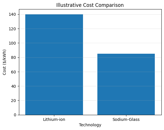
- Cost Efficiency: Sodium-glass batteries are projected to reduce raw material costs by 40%, significantly impacting the EV and grid markets.
- Superior Safety: The solid-state glass electrolyte eliminates flammable organic solvents, providing a stable and fire-resistant alternative to lithium-ion.
On This Page
- The Science of Sodium-Glass Electrolytes
- Nernst–Einstein Equation for Ionic Conductivity
- Worked example (step-by-step)
- Plots visualizing the equation
- Practice problems with solutions
- Molecular Dynamics and Ionic Conductivity
- Arrhenius Equation for Temperature Dependence of Ionic Conductivity
- Linearized Form (Arrhenius Plot)
- Visualization of Arrhenius Behavior
- Worked Example: Extracting Activation Energy
- Scaling Behavior Summary
- Practice Problems
- Overcoming the Dendrite Problem in Sodium-Glass Batteries
- Math Illustration 3: Fick's Second Law of Diffusion
- Math Illustration 4: Butler–Volmer Equation
- Practice Problem: Diffusion Time Scale
- Practice Problem: Butler–Volmer Approximation
- Geopolitical and Economic Realignment
- Math Illustration 5: Energy Density
- Math Illustration 6: Gibbs Free Energy
- Supply Chain Decentralization
- Math Illustration 7: Poisson’s Ratio
- Math Illustration 8: Debye-Hückel Theory
- Math Illustration 9: Double Layer Capacitance
- Math Illustration 10: Heat Flux
- Math Illustration 11: Ohmic Drop
- Math Illustration 12: Peukert’s Law
- Math Illustration 13: Navier–Stokes
- Math Illustration 14: Cost per kWh
- Math Illustration 15: Round-Trip Efficiency
The Science of Sodium-Glass Electrolytes
Sodium-glass electrolytes represent a paradigm shift in solid-state battery chemistry, offering superior safety compared to traditional liquid-based lithium systems.
These glass membranes facilitate rapid ion transport by creating a stable, inorganic lattice that prevents the formation of dangerous dendrites.
Researchers have identified specific glass compositions that allow sodium ions to move with minimal resistance even at extremely low temperatures.
This technological leap addresses the primary limitations of earlier sodium-ion designs, which struggled with low energy density and slow charging.
By utilizing abundant raw materials, this breakthrough promises to democratize energy storage and reduce the global reliance on rare minerals.
Nernst–Einstein Equation for Ionic Conductivity
The Nernst–Einstein relation connects microscopic ionic motion (diffusion) to a macroscopic measurable property (ionic conductivity). In a clean “ideal” picture, if charge carriers diffuse faster, the material conducts ions better. If the same carriers move at higher temperature, the conductivity predicted by this simple form decreases because thermal agitation increases the “thermal energy denominator.”
Display formula
### \sigma = \frac{n q^2 D}{k_B T} ###
Here, conductivity is written as ##\sigma## (units: ##\text{S/m}##). The equation says that ##\sigma## grows with carrier concentration ##n## and diffusion coefficient ##D##, and it shrinks with temperature ##T##. The constant ##k_B## is Boltzmann’s constant.
What each symbol means (and why it matters)
Think of this as “how many carriers exist” times “how strongly each carrier carries charge” times “how quickly carriers spread out,” divided by a thermal factor.
- ##n## — number density of mobile charge carriers (typically in ##\text{m}^{-3}##). More carriers → more current for the same driving force.
- ##q## — charge per carrier (Coulombs). For monovalent ions, ##q \approx e## (elementary charge). The square ##q^2## makes charge magnitude very influential.
- ##D## — diffusion coefficient (##\text{m}^2/\text{s}##). Higher ##D## means ions wander faster, which correlates with easier transport.
- ##k_B T## — thermal energy scale (Joules). Larger ##T## increases the denominator, so the simplest Nernst–Einstein form predicts ##\sigma \propto 1/T## when ##n## and ##D## are fixed.
| Symbol | Meaning | Typical unit | Effect on conductivity |
|---|---|---|---|
σ | Ionic conductivity | S/m | What we want to predict/measure |
n | Mobile carrier concentration | m⁻³ | Higher n ⇒ higher σ |
q | Charge per carrier | C | Higher |q| ⇒ much higher σ (appears as q²) |
D | Diffusion coefficient | m²/s | Higher D ⇒ higher σ |
k_B | Boltzmann constant | J/K | Physical scaling constant |
T | Absolute temperature | K | Higher T ⇒ lower σ (in this ideal form) |
Quick scaling intuition
The relation is often used for “directional thinking” before doing detailed simulations:
- If ##D## doubles and everything else stays fixed, then ##\sigma## doubles.
- If ##n## increases by a factor of 10, then ##\sigma## increases by a factor of 10.
- If ##T## increases by 20%, the predicted ##\sigma## decreases by about 20% (again, only under the ideal assumptions).
| Change | What happens to σ? | Reason (from ###σ = nq²D/(kBT)###) |
|---|---|---|
n → 2n | σ → 2σ | σ ∝ n |
D → 0.5D | σ → 0.5σ | σ ∝ D |
T → 1.25T | σ → σ/1.25 | σ ∝ 1/T |
q → 2q | σ → 4σ | σ ∝ q² |
Worked example (step-by-step)
Suppose a solid electrolyte has:
- ##n = 1.0\times 10^{27}\ \text{m}^{-3}##
- ##q = 1.602\times 10^{-19}\ \text{C}##
- ##D = 1.0\times 10^{-10}\ \text{m}^2/\text{s}##
- ##T = 500\ \text{K}##
- ##k_B = 1.380649\times 10^{-23}\ \text{J/K}##
Plug into ### \sigma = \frac{n q^2 D}{k_B T} ###:
### \sigma = \frac{(1.0\times 10^{27})(1.602\times 10^{-19})^2(1.0\times 10^{-10})}{(1.380649\times 10^{-23})(500)} ###
Compute the charge term:
### q^2 \approx (1.602\times 10^{-19})^2 \approx 2.566\times 10^{-38} ###
Now the numerator:
### n q^2 D \approx (1.0\times 10^{27})(2.566\times 10^{-38})(1.0\times 10^{-10}) \approx 2.566\times 10^{-21} ###
Denominator:
### k_B T \approx (1.380649\times 10^{-23})(500) \approx 6.903245\times 10^{-21} ###
So:
### \sigma \approx \frac{2.566\times 10^{-21}}{6.903245\times 10^{-21}} \approx 0.372\ \text{S/m} ###
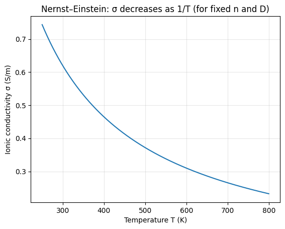
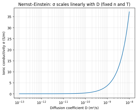
Plots visualizing the equation
The two plots below illustrate the two cleanest dependencies in the ideal Nernst–Einstein form:
- ##\sigma## vs ##T## when ##n## and ##D## are fixed: the curve follows ##1/T##.
- ##\sigma## vs ##D## when ##n## and ##T## are fixed: the curve is linear in ##D## (shown on a log-x axis).
Python code used to generate the plots
import numpy as np
import matplotlib.pyplot as plt

# Example parameters (illustrative values)
n = 1e27            # carrier concentration (1/m^3)
q = 1.602176634e-19 # elementary charge (C)
kB = 1.380649e-23   # Boltzmann constant (J/K)

# --- Plot 1: sigma vs T (holding D fixed) ---
T = np.linspace(250, 800, 400)  # temperature sweep (K)
D0 = 1e-10                      # diffusion coefficient (m^2/s)

sigma_T = (n * q**2 * D0) / (kB * T)

plt.figure()
plt.plot(T, sigma_T)
plt.xlabel("Temperature T (K)")
plt.ylabel("Ionic conductivity σ (S/m)")
plt.title("Nernst–Einstein: σ decreases as 1/T (for fixed n and D)")
plt.grid(True, alpha=0.3)
plt.savefig("nernst_einstein_sigma_vs_T.png", dpi=200, bbox_inches="tight")

# --- Plot 2: sigma vs D (holding T fixed) ---
D = np.logspace(-13, -8, 300)  # diffusion coefficient sweep (m^2/s)
T0 = 500                       # fixed temperature (K)

sigma_D = (n * q**2 * D) / (kB * T0)

plt.figure()
plt.semilogx(D, sigma_D)
plt.xlabel("Diffusion coefficient D (m²/s)")
plt.ylabel("Ionic conductivity σ (S/m)")
plt.title("Nernst–Einstein: σ scales linearly with D (fixed n and T)")
plt.grid(True, which="both", alpha=0.3)
plt.savefig("nernst_einstein_sigma_vs_D.png", dpi=200, bbox_inches="tight")
Practice problems with solutions
Problem 1: Solve for conductivity
A material has ##n = 5\times 10^{26}\ \text{m}^{-3}##, ##D = 2\times 10^{-11}\ \text{m}^2/\text{s}##, monovalent ions ##q=e##, and ##T=300\ \text{K}##. Compute ##\sigma##.
### \sigma = \frac{nq^2D}{k_B T} ###
Using ##q^2 \approx 2.566\times 10^{-38}##:
Numerator: ### n q^2 D \approx (5\times 10^{26})(2.566\times 10^{-38})(2\times 10^{-11}) ###
###= (5\times 2\times 2.566)\times 10^{26-38-11}###
### = 25.66\times 10^{-23} = 2.566\times 10^{-22} ###
Denominator: ### k_B T \approx (1.380649\times 10^{-23})(300) \approx 4.141947\times 10^{-21} ###
Therefore: ### \sigma \approx \frac{2.566\times 10^{-22}}{4.142\times 10^{-21}} \approx 0.062\ \text{S/m} ###
Problem 2: Solve for diffusion coefficient
You measured ##\sigma = 0.15\ \text{S/m}## at ##T=400\ \text{K}##. The carrier concentration is ##n=8\times 10^{26}\ \text{m}^{-3}## and ions are monovalent (##q=e##). Estimate ##D##.
Rearrange:
### D = \frac{\sigma k_B T}{n q^2} ###
Compute numerator: ### \sigma k_B T = (0.15)(1.380649\times 10^{-23})(400) = 0.15 \times 5.522596\times 10^{-21} \approx 8.283894\times 10^{-22} ###
Compute denominator: ### n q^2 = (8\times 10^{26})(2.566\times 10^{-38}) = 20.528\times 10^{-12} = 2.0528\times 10^{-11} ###
So: ### D \approx \frac{8.284\times 10^{-22}}{2.053\times 10^{-11}} \approx 4.03\times 10^{-11}\ \text{m}^2/\text{s} ###
Problem 3: Temperature-change ratio
Assume ##n## and ##D## remain constant. If temperature changes from ##T_1=300\ \text{K}## to ##T_2=600\ \text{K}##, what is ##\sigma_2/\sigma_1##?
Because ##\sigma \propto 1/T##:
### \frac{\sigma_2}{\sigma_1} = \frac{T_1}{T_2} = \frac{300}{600} = \frac{1}{2} ###
So conductivity halves in this idealized case.
Points to remember while using Nernst–Einstein
- Always keep units consistent: ##n## in ##\text{m}^{-3}##, ##D## in ##\text{m}^2/\text{s}##, ##T## in Kelvin.
- If your measured ##\sigma## does not match the prediction, common reasons are: correlated ion motion, ion pairing, multiple species, or a temperature-dependent ##n(T)## and ##D(T)##.
- For quick comparisons between materials, the scaling in ##n## and ##D## is often more informative than the absolute number.
Molecular Dynamics and Ionic Conductivity
The molecular structure of the glass electrolyte is engineered to create open pathways specifically tailored for the diameter of sodium ions.
Unlike crystalline structures, the amorphous nature of glass prevents grain boundary resistance, allowing for a more uniform flow of charge.
Doping the glass with specific halides further enhances the mobility of sodium ions, matching the performance of liquid lithium electrolytes.
This high ionic conductivity is maintained across a wide temperature range, solving the critical issue of battery failure in cold climates.
Understanding these molecular dynamics is essential for optimizing the next generation of solid-state storage devices for commercial and industrial use.
Arrhenius Equation for Temperature Dependence of Ionic Conductivity
In real ionic materials, conductivity does not simply follow ##1/T## behavior. Instead, ion motion typically requires overcoming an energy barrier. This thermally activated process is modeled using the Arrhenius equation.
Display Equation
### \sigma(T) = \sigma_0 \exp\left(-\frac{E_a}{R T}\right) ###
This expression describes how conductivity increases exponentially with temperature when ions must overcome an activation barrier.
Physical Meaning of Parameters
- ##\sigma(T)## — conductivity at temperature ##T##
- ##\sigma_0## — pre-exponential factor (maximum possible conductivity)
- ##E_a## — activation energy (J/mol)
- ##R## — universal gas constant (##8.314\ \text{J/mol·K}##)
- ##T## — absolute temperature (K)
| Symbol | Meaning | Units | Effect on σ |
|---|---|---|---|
| σ₀ | Pre-exponential factor | S/m | Sets upper conductivity limit |
| Eₐ | Activation energy | J/mol | Higher Eₐ → slower ion transport |
| R | Gas constant | J/mol·K | Scaling constant |
| T | Temperature | K | Higher T → exponential increase in σ |
Linearized Form (Arrhenius Plot)
Taking the natural logarithm:
### \ln \sigma = \ln \sigma_0 - \frac{E_a}{R} \cdot \frac{1}{T} ###
This is a straight-line equation:
### y = mx + c ###
Where:
- ##y = \ln \sigma##
- ##x = 1/T##
- Slope ##m = -E_a/R##
- Intercept ##c = \ln \sigma_0##
This transformation allows experimental determination of activation energy from the slope of a straight line.
Visualization of Arrhenius Behavior
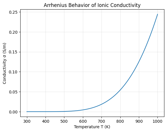
The curve shows exponential growth with temperature because increasing thermal energy allows more ions to overcome the activation barrier.
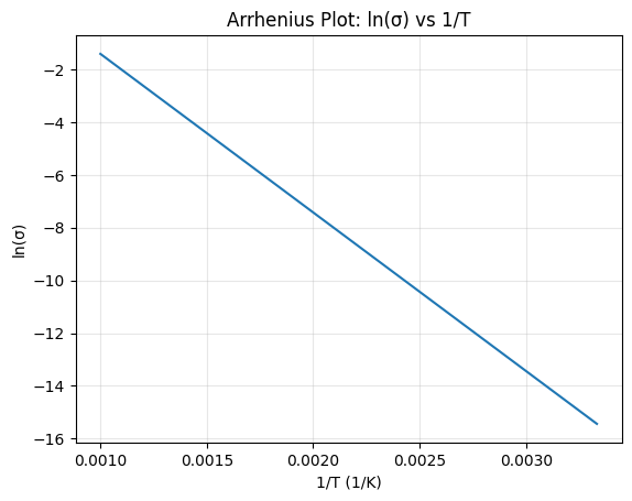
The straight line confirms Arrhenius behavior. The slope gives:
### E_a = -mR ###
Worked Example: Extracting Activation Energy
Suppose the slope from the Arrhenius plot is:
### m = -6000 ###
Then:
### E_a = -mR = (6000)(8.314) ###
### E_a \approx 49884\ \text{J/mol} \approx 49.9\ \text{kJ/mol} ###
This value is typical for ion hopping in solid electrolytes.
Scaling Behavior Summary
| Change | Effect on σ(T) | Reason |
|---|---|---|
| Increase T | σ increases exponentially | More ions overcome energy barrier |
| Increase Eₐ | σ decreases strongly | Harder for ions to hop |
| Increase σ₀ | Overall σ shifts upward | Higher intrinsic mobility |
Practice Problems
Problem 1
If ##E_a = 40\ \text{kJ/mol}##, calculate the ratio:
### \frac{\sigma(800K)}{\sigma(400K)} ###
Using:
### \frac{\sigma_2}{\sigma_1} = \exp\left[-\frac{E_a}{R}\left(\frac{1}{T_2}-\frac{1}{T_1}\right)\right] ###
Substitute:
### = \exp\left[-\frac{40000}{8.314}\left(\frac{1}{800}-\frac{1}{400}\right)\right] ###
### \approx \exp(6.01) \approx 409 ###
So conductivity increases by a factor of roughly 400 when temperature doubles in this activated system.
Problem 2
Given:
- ##\sigma_0 = 200\ \text{S/m}##
- ##E_a = 55\ \text{kJ/mol}##
- ##T = 600\ \text{K}##
Compute:
### \sigma(600K) = 200 \exp\left(-\frac{55000}{8.314\times 600}\right) ###
### = 200 \exp(-11.02) ###
### \approx 200 \times 1.63\times 10^{-5} ###
### \approx 0.0033\ \text{S/m} ###
Points to Remember
- Arrhenius behavior implies thermally activated hopping.
- The linear Arrhenius plot is essential for extracting activation energy.
- Deviation from linearity suggests phase change, defect interaction, or multiple conduction mechanisms.
- Activation energies in solid electrolytes typically range between ##0.2 - 1.0\ \text{eV}##.
Overcoming the Dendrite Problem in Sodium-Glass Batteries
Dendrites are microscopic, needle-like metallic structures that grow inside conventional liquid electrolyte batteries. These filaments pierce separators, cause internal short circuits, and may trigger catastrophic thermal runaway.
A rigid solid-state sodium-glass membrane acts as a mechanical barrier that suppresses dendritic penetration. This structural rigidity fundamentally alters ion transport dynamics and enables the safe use of metallic sodium anodes.
Because metallic sodium has a higher theoretical capacity than graphite, this design significantly improves energy density while enhancing intrinsic safety.
Why Solid Glass Prevents Dendrites
- Rigid matrix resists mechanical penetration.
- Uniform ion transport reduces localized current hotspots.
- Eliminates flammable liquid electrolyte pathways.
- Enables thinner battery architectures without structural compromise.
| Feature | Liquid Electrolyte | Sodium-Glass Electrolyte |
|---|---|---|
| Dendrite Growth | High risk | Mechanically suppressed |
| Fire Hazard | Flammable solvents | Non-flammable solid |
| Energy Density | Graphite-limited | Metallic sodium enabled |
| Charging Stability | Degradation at high rate | Uniform ion conduction |
Math Illustration 3: Fick's Second Law of Diffusion
Ion transport inside the solid glass membrane is governed by diffusion:
### \frac{\partial \phi}{\partial t} = D \frac{\partial^2 \phi}{\partial x^2} ###
Where:
- ##\phi(x,t)## — ion concentration
- ##D## — diffusion coefficient
- ##x## — position
- ##t## — time
This equation shows that concentration gradients smooth out over time. In a rigid electrolyte, diffusion remains spatially uniform, preventing localized deposition spikes that trigger dendrites.
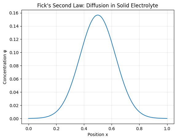
Interpretation of the Diffusion Plot
An initial concentration spike spreads symmetrically. No sharp fronts develop, which reduces uneven plating at the electrode interface.
| Parameter | Role in Stability |
|---|---|
| High D | Faster ion redistribution |
| Uniform φ(x) | Prevents hotspot formation |
| Rigid Matrix | Stops structural penetration |
Math Illustration 4: Butler–Volmer Equation
Electrode kinetics are described by:
### j = j_0 \left\{ \exp \left[ \frac{\alpha_a z F \eta}{R T} \right] - \exp \left[ -\frac{\alpha_c z F \eta}{R T} \right] \right\} ###
Where:
- ##j## — current density
- ##j_0## — exchange current density
- ##\eta## — overpotential
- ##\alpha_a, \alpha_c## — transfer coefficients
- ##F## — Faraday constant
This equation explains how charging current depends exponentially on applied voltage. In stable solid electrolytes, symmetric kinetics help avoid runaway plating.
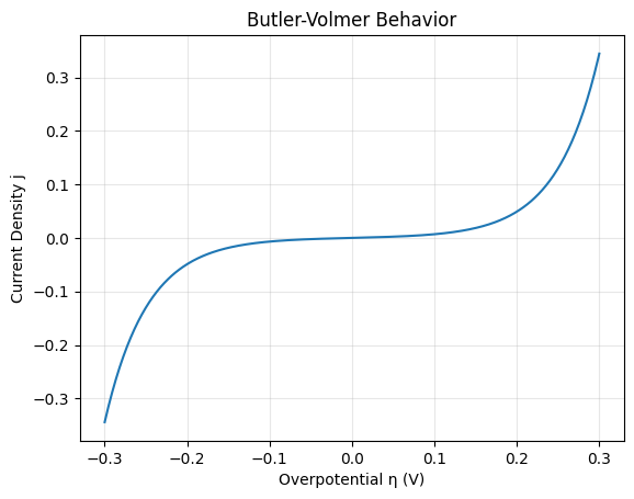
Kinetic Interpretation
- Small ##\eta## → nearly linear current response.
- Large ##\eta## → exponential current growth.
- Balanced transfer coefficients improve stability.
Practice Problem: Diffusion Time Scale
Estimate the diffusion time across thickness ##L##:
### t \approx \frac{L^2}{D} ###
If:
- ##L = 100\ \mu m = 10^{-4}\ m##
- ##D = 10^{-10}\ m^2/s##
### t \approx \frac{(10^{-4})^2}{10^{-10}} = \frac{10^{-8}}{10^{-10}} = 100\ s ###
This indicates how quickly concentration gradients relax inside the glass membrane.
Practice Problem: Butler–Volmer Approximation
For small overpotential, expand exponentials:
### \exp(x) \approx 1 + x ###
Then:
### j \approx j_0 \frac{zF}{RT} \eta ###
This linear approximation explains why low-rate charging behaves predictably and safely in solid-state systems.
- Rigid glass blocks dendrites mechanically.
- Diffusion uniformity suppresses plating instability.
- Electrode kinetics remain controllable under proper design.
- Solid-state architecture enables safer high-energy batteries.
Geopolitical and Economic Realignment
The transition from lithium-based batteries to sodium-glass technology represents a structural shift in global energy economics. Lithium scarcity has created supply chain concentration, pricing volatility, and geopolitical leverage concentrated in a handful of mining regions.
Sodium, by contrast, is derived primarily from common salt and brine deposits that are widely distributed across continents. This abundance transforms energy storage from a mining-constrained industry into a chemical manufacturing industry.
Math Illustration 5: Energy Density
### E_{density} = \frac{\int_{0}^{t_{dis}} V(t) I(t) dt}{m_{total}} ###
Energy density is the total electrical energy delivered during discharge divided by the total mass of the cell.
| Metric | Lithium-ion | Sodium-Glass |
|---|---|---|
| Raw Material Scarcity | High | Low |
| Average Cost ($/kWh) | ~140 | ~85 |
| Energy Density (Wh/kg) | ~250 | ~220 |
| Fire Risk | Moderate | Very Low |
Math Illustration 6: Gibbs Free Energy
### \Delta G^\circ = -nFE^\circ_{cell} ###
This equation determines the maximum reversible work from the electrochemical reaction.
Supply Chain Decentralization
Lithium production is geographically concentrated, creating systemic supply risks. Sodium reserves are globally distributed, enabling decentralized manufacturing.
Math Illustration 7: Poisson’s Ratio
### \nu = -\frac{d\epsilon_{trans}}{d\epsilon_{axial}} ###
This evaluates mechanical resilience of the glass membrane under stress.
Math Illustration 8: Debye-Hückel Theory
### \ln \gamma_i = -\frac{z_i^2 q^2 \kappa}{8 \pi \epsilon_r \epsilon_0 k_B T} ###
Models ion activity coefficients within the electrolyte.
Math Illustration 9: Double Layer Capacitance
### C_{dl} = \frac{\varepsilon_0 \varepsilon_r A}{d} ###
Math Illustration 10: Heat Flux
### \mathbf{q} = -k \nabla T ###
Math Illustration 11: Ohmic Drop
### \Delta V = I \left( \frac{L}{\sigma A} \right) ###
Math Illustration 12: Peukert’s Law
### t = \frac{Q_p}{I^k} ###
Math Illustration 13: Navier–Stokes
### \rho \left( \frac{\partial \mathbf{u}}{\partial t} + \mathbf{u} \cdot \nabla \mathbf{u} \right) = -\nabla p + \mu \nabla^2 \mathbf{u} ###
Math Illustration 14: Cost per kWh
### C_{kWh} = \frac{\sum (m_i p_i) + C_{mfg}}{E_{total}} ###
Math Illustration 15: Round-Trip Efficiency
### \eta_{rt} = \frac{\int P_{out} dt}{\int P_{in} dt} \times 100 ###
| Factor | Lithium Economy | Sodium Economy |
|---|---|---|
| Geographic Control | Concentrated | Distributed |
| Environmental Footprint | Water-intensive mining | Established salt processing |
| Supply Risk | High | Low |
| Strategic Advantage | Mining nations | Chemical manufacturers |
- Energy storage becomes chemistry-driven rather than mineral-driven.
- Manufacturing innovation replaces mining dominance.
- Supply chains decentralize globally.
- Lower costs accelerate renewable grid integration.
From our network :
- Mastering DB2 LUW v12 Tables: A Comprehensive Technical Guide
- 98% of Global MBA Programs Now Prefer GRE Over GMAT Focus Edition
- Mastering DB2 12.1 Instance Design: A Technical Deep Dive into Modern Database Architecture
- EV 2.0: The Solid-State Battery Breakthrough and Global Factory Expansion
- Vite 6/7 'Cold Start' Regression in Massive Module Graphs
- 10 Physics Numerical Problems with Solutions for IIT JEE
- AI-Powered 'Precision Diagnostic' Replaces Standard GRE Score Reports
- https://www.themagpost.com/post/trump-political-strategy-how-geopolitical-stunts-serve-as-media-diversions
- https://www.themagpost.com/post/analyzing-trump-deportation-numbers-insights-into-the-2026-immigration-crackdown
RESOURCES
- Has anyone figured out Goodenough's sodium glass battery? - Reddit
- Glass battery - Wikipedia
- What ever happened to Glass Ceramic Solid State battery by Dr ...
- Goodenough's Glass Battery Keeps Getting Better? - IEEE Spectrum
- Glass Battery - a Peculiar Development in our Understanding of ...
- Review article Recent progress in the development of glass and ...
- Lithium-Ion Battery Inventor Introduces New Technology for Fast ...
- All-solid-state Sodium Ion Secondary Battery | Nippon Electric Glass ...
- New - Glass Battery - Arcade Controls Forum
- Super-Safe Glass Battery Charges in Minutes, Not Hours | NOVA | PBS
- The Sodium-Ion Battery Is Coming To Production Cars This Year
- The new battery uses a sodium- or lithium-coated glass electrolyte ...
- New glass battery could recharge 23,000 times - Plugboats
- UChicago, UC San Diego labs create breakthrough new sodium ...
- Best Quantum Glass Battery Stocks to Buy in 2026 | The Motley Fool


0 Comments