
The slope-intercept form is a foundational concept that underpins much of algebra and graphing. It's vital to know how this form works because it's instrumental in interpreting linear functions and graphing lines effectively. When you grasp the slope-intercept form, you unlock the door to solving equations that illustrate relationships between various variables in a straightforward manner. Understanding this form is like having a roadmap that guides you through the complexities of linear equations.
On This Page
- What is the Slope-Intercept Form?
- How to Derive and Work with the Slope-Intercept Form
- Examples of the Slope-Intercept Form
- Applications of Slope-Intercept Form
- Final Solution
- Below are a few additional problems related to the slope-intercept form.
- Problem 1: Find the slope of the line given by ##y = 3x - 7##.
- Problem 2: Write the slope-intercept form of a line with slope 4 and passing through the point (0, 5).
- Problem 3: Convert the equation ##2x + 3y = 6## into slope-intercept form.
- Problem 4: Determine the slope and y-intercept from the function ##y = -5x + 10##.
- Problem 5: If the slope of a line is ##\frac{1}{4}## and the y-intercept is -3, write the equation.
- We also Published
- RESOURCES
At the core of the slope-intercept form is the equation written as y = mx + b, where 'm' signifies the slope and 'b' represents the y-intercept. This structure not only makes plotting graphs simpler but also allows you to easily analyze how a line behaves. For instance, a positive slope indicates a rise from left to right, while a negative slope suggests a decline. Becoming familiar with these elements will significantly enhance your ability to graph linear functions and understand their real-world applications.
More from me
This blog post delves into the slope-intercept form of a line, a fundamental concept in algebra and graphing. Understanding this form is crucial for interpreting linear functions, graphing lines, and solving equations that describe relationships between variables.
What is the Slope-Intercept Form?
The slope-intercept form of a linear equation is expressed as ##y = mx + b##, where ##m## represents the slope of the line and ##b## indicates the y-intercept. The slope, ##m##, is calculated as the ratio of the rise over the run between any two points on the line, which gives us the steepness of the line. The y-intercept, ##b##, is the point where the line crosses the y-axis, providing us with critical information about the graph.
This form of a linear equation is particularly useful because it allows for easy plotting of the line on a Cartesian plane. By identifying the slope and y-intercept, we can determine actively how the line behaves. For example, a positive slope means the line ascends from left to right, while a negative slope indicates it descends. Understanding both of these components is essential for graphing linear functions accurately.
How to Derive and Work with the Slope-Intercept Form
Deriving the Equation
To derive the slope-intercept form, we start with the general formula of a line and isolate ##y##. Suppose you have a standard equation in point-slope form: ##y - y_1 = m(x - x_1)##. Rearranging this leads to: ### y = mx + (y_1 - mx_1) ###. The term ##(y_1 - mx_1)## is equivalent to the y-intercept, ##b##, thus reinforcing the slope-intercept form of a line used in coordinate geometry.
Graphical Representation of Slope-Intercept Form
To visualize the slope-intercept form, let’s take an example. Consider the equation ##y = 2x + 3##. Here, the slope, ##m = 2##, indicates that for each unit increase in x, y increases by 2 units. The y-intercept, ##b = 3##, tells us that the line crosses the y-axis at (0,3). By plotting these points and using the slope to find additional coordinates, you can graph the line accurately and understand the relationships depicted in linear equations.
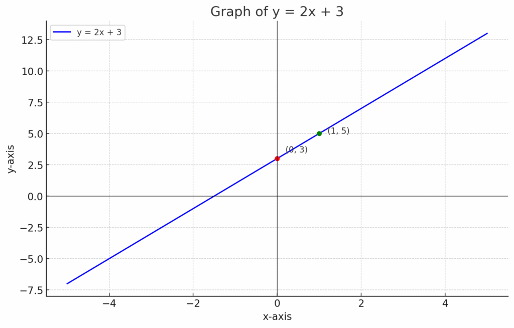
Here's the graph of the equation ##y=2x+3y## . The red point marks the y-intercept at ##(0,3)##, and the green point at ##(1,5)## shows how the slope of 2 moves the line: one unit to the right in xxx results in a two-unit increase in ##y##. This visual reinforces how slope and intercept define the behavior of a linear equation.
Examples of the Slope-Intercept Form
Example 1: Given a Slope and Y-Intercept
Suppose we have the equation ##y = -\frac{1}{2}x + 4##. Here, the slope is ##-\frac{1}{2}##, which indicates that the line descends with a gentle slope. The y-intercept is 4, meaning the line crosses the y-axis at the point (0,4). You can graph this function to visually confirm the negative slope.
Example 2: Finding Slope and Y-Intercept
If we have two points, for example, (2,5) and (6,9), we can find the slope and y-intercept. The slope, calculated as ##m = \frac{y_2 - y_1}{x_2 - x_1} = \frac{9 - 5}{6 - 2} = 1##. We can then use one point to find the intercept. Substituting into the equation ### y - 5 = 1(x - 2) ### leads us to the slope-intercept form: ##y = x + 3##.
Applications of Slope-Intercept Form
Real-World Applications
The slope-intercept form is prevalent in various fields including economics, physics, and social sciences. For instance, it can describe demand and supply curves in economics, which helps businesses and analysts understand market behaviors and predict trends. Graphical interpretation is crucial for making forecasts based on historical data.
Importance in Calculus and Beyond
Understanding the slope-intercept form also lays the foundation for more advanced concepts in calculus and linear algebra. Recognizing how lines interact through slopes and intercepts paves the way for grasping tangent lines, optimization problems, and linear regression analysis, essential for predictive modeling. The slope is a derivative concept that plays a critical role in calculus.
Final Solution
The slope-intercept form provides a clear method for expressing linear functions in mathematics with the equation: ##y = mx + b##. With this knowledge, one can quickly determine how to graph linear equations and their behavior in relation to x and y coordinates. This fundamental equation serves as a basis for further exploration in mathematics and its applications.
Below are a few additional problems related to the slope-intercept form.
Problem 1: Find the slope of the line given by ##y = 3x - 7##.
The slope is ##m = 3##.
Problem 2: Write the slope-intercept form of a line with slope 4 and passing through the point (0, 5).
The equation is ##y = 4x + 5##.
Problem 3: Convert the equation ##2x + 3y = 6## into slope-intercept form.
The slope-intercept form is ##y = -\frac{2}{3}x + 2##.
Problem 4: Determine the slope and y-intercept from the function ##y = -5x + 10##.
The slope is ##m = -5## and the y-intercept is ##b = 10##.
Problem 5: If the slope of a line is ##\frac{1}{4}## and the y-intercept is -3, write the equation.
The equation is ##y = \frac{1}{4}x - 3##.
We also Published
RESOURCES
- Introduction to Linear Equations | Algebra (article) | Khan Academy
- Intro to Linear Equation Forms (y=mx+b) | Algebra (video) | Khan ...
- How long do you spend on learning linear equation forms? : r/matheducation
- Forms of a Linear Equation: An Overview
- Origins of Linear Equation Forms: A Historical Perspective : r/AskHistorians
- Linear Equations Calculator (y-intercept graph Calculator)
- Write an Equation from a Graph | Algebra 1 Practice - IXL
- Understanding Linear Equation Forms - Mathplanet
- Graphing Linear Equations (Algebra 1 practice) - IXL
- Straight-Line Equations: Understanding Linear Equation Forms | Purplemath


0 Comments