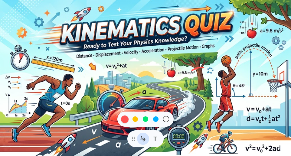
Motion in One Dimension forms the foundational block in understanding the Physics of movement. This topic delves into the specifics of how objects move in a straight line under the influence of various forces. By exploring the key concepts of displacement, velocity, and acceleration, one can grasp how these parameters interrelate to describe the kinematic motion of particles or bodies in a single-dimensional plane.

Understanding Motion in One Dimension

Motion in One Dimension, also known as Rectilinear Motion, focuses on the movement of objects along a straight path. This type of motion simplifies the analysis of movement as it restricts the scenario to a single axis, usually the x-axis. To comprehend this, we examine three primary components: displacement, velocity, and acceleration.

Displacement

Displacement refers to the change in position of an object. It is a vector quantity, meaning it has both magnitude and direction. If an object moves from position \(x_1\) to \(x_2\), the displacement \( \Delta x \) is given by:
\[
\Delta x = x_2 – x_1
\]
This provides a clear understanding of how far and in which direction the object has travelled.

Velocity

Velocity signifies the rate of change of displacement with respect to time. It also is a vector quantity. The average velocity \(v_{\text{avg}}\) can be calculated by:
\[
v_{\text{avg}} = \frac{\Delta x}{\Delta t}
\]
where \( \Delta x \) is displacement and \( \Delta t \) is the time interval. Instantaneous velocity refers to the velocity at a specific point in time, derived as the limit of the average velocity as the time interval approaches zero:
\[
v = \lim_{\Delta t \to 0} \frac{\Delta x}{\Delta t} = \frac{dx}{dt}
\]

Acceleration

Acceleration denotes the rate of change of velocity with time. This vector quantity provides insights into how quickly an object speeds up or slows down along its path. The average acceleration \(a_{\text{avg}}\) is expressed as:
\[
a_{\text{avg}} = \frac{\Delta v}{\Delta t}
\]
Similarly, instantaneous acceleration is the derivative of velocity with respect to time:
\[
a = \frac{dv}{dt}
\]

“The definition of acceleration is found in the analysis of the change in the velocity vector, providing a powerful tool for predicting future motion attributes of objects.”

Equations of Motion

Key equations of motion are pivotal for solving problems regarding motion in one dimension. These equations interlink displacement, velocity, acceleration, and time, anchoring our understanding to predictable mathematical relationships. They are:

First Equation of Motion

The first equation relates velocity and acceleration:
\[
v = u + at
\]
where \( u \) is the initial velocity, \( v \) is the final velocity, \( a \) is acceleration, and \( t \) is time.

Second Equation of Motion

The second equation expresses displacement in terms of velocity and time:
\[
s = ut + \frac{1}{2}at^2
\]
Here, \( s \) represents displacement.

Third Equation of Motion

The third equation connects initial velocity, final velocity, acceleration, and displacement:
\[
v^2 = u^2 + 2as
\]

“These kinematic equations provide vital methodologies to determine unknown variables in one-dimensional motion.”

Practical Examples in Motion

To solidify understanding, practical examples help illustrate the theoretical concepts. Let’s consider an object under constant acceleration.

Example 1: Dropping an Object

Calculate the final velocity of an object dropped from rest after 5 seconds. Given that the acceleration due to gravity \( g \) is \( 9.8 m/s^2 \):
\[
v = u + at = 0 + (9.8)(5) = 49 m/s
\]

Example 2: Car Braking

A car travelling at 20 m/s comes to a stop in 4 seconds. Calculate the acceleration. Utilizing the first equation of motion:
\[
v = u + at \implies 0 = 20 + (a)(4) \implies a = -5 m/s^2
\]

Example 3: Distance Covered by a Moving Object

A vehicle accelerates from rest with an acceleration of \( 3 m/s^2 \) for 8 seconds. Calculate the distance covered:
\[
s = ut + \frac{1}{2}at^2 = 0\cdot8 + \frac{1}{2}\cdot3\cdot8^2 = 96 \text{ meters}
\]

# Python code for calculating distance
initial_velocity = 0
acceleration = 3
time = 8
distance = (initial_velocity * time) + (0.5 * acceleration * time**2)
print(distance)

96

Graphs of Motion

Graphs provide a compelling way to analyze one-dimensional motion. By plotting displacement-time, velocity-time, and acceleration-time graphs, one can visualize the trends and derive information about the object’s motion.

Displacement-Time Graph

A straight line on this graph indicates constant velocity. A curved line implies changing velocity, denoting acceleration or deceleration.

Velocity-Time Graph

A horizontal line represents constant velocity. The slope of this line gives acceleration. A line with a positive slope indicates acceleration, while a negative slope indicates deceleration.

Acceleration-Time Graph

This graph shows how acceleration changes over time.

Applications in Real Life

Understanding motion in one dimension has practical applications in multiple fields including transportation, sports, engineering, and safety mechanisms.

Transportation: Calculation of stopping distances, design of road safety features, and optimization of vehicle performance rely heavily on these principles.

Sports: Athletic performance analysis leverages these concepts to enhance training methodologies and improve results.

Engineering: Mechanical designs, structure integrity assessments, and dynamics computations depend on accurate predictions of motion.

Safety Mechanisms: Safety mechanisms in vehicles and machinery, like airbags and automated emergency braking, utilize concepts from one-dimensional motion to function effectively.

“Mastery of these fundamental principles opens avenues for innovation and safety implementations in various sectors.”