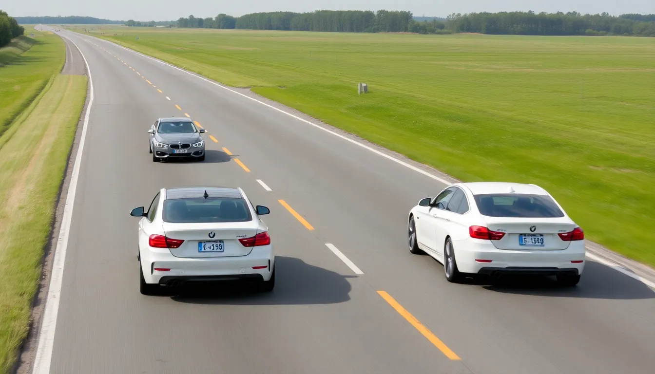
When we analyze relative motion, we are essentially studying how objects move in relation to each other. This concept is fundamental to understanding physics, allowing us to solve complex problems. In this post, we will break down how to determine the meeting point of two cars, using the principles of kinematics to predict their interactions accurately.
On This Page
Read More
To fully grasp how objects move in relation to each other, we must delve into the core principles of kinematics. This exploration of motion extends beyond simple calculations; it involves a detailed understanding of position, velocity, and acceleration over time. Our focus will be on understanding the concept of relative motion as we compare the movements of two cars, a classic problem in physics that demonstrates the power of mathematical modeling.
Cracking the Code: Deconstructing the Problem
Let's start by setting the stage: Car A begins its journey at the zero mark, accelerating steadily, while Car B begins behind it, initially moving faster but slowing down. This scenario sets up a dynamic interplay that challenges us to find when and where these two cars intersect. The challenge lies in translating the narrative of their movements into mathematical equations, allowing us to predict their future positions. This involves creating position functions for each car, which we will then use to determine the time and location of their meeting.
Mapping the Motion: Car A's Journey
Car A starts at rest and accelerates. The motion can be divided into two phases: the initial acceleration phase and the subsequent constant velocity phase. To write a position function, we must apply the equations of motion. During the acceleration phase (0 ≤ t ≤ 8 s), the position is determined by the equation ##x_A(t) = v_0t + (1/2)at^2##, where ##v_0## is the initial velocity, and 'a' is the acceleration. After 8 seconds, the car moves at a constant speed, and the position function will be a linear equation.
Let's break down Car A's motion. The initial velocity, ##v_0##, is 25 m/s, and the acceleration, 'a', is 1.5 m/s². Applying these values, we get ##x_A(t) = 25t + (1/2)(1.5)t^2##. After the acceleration phase, we use the final velocity to determine the position. At t = 8 s, the car's position and velocity transition to a constant speed phase. The position function must then be adjusted to account for this change, ensuring we accurately model the car's movement over time.
Mapping the Motion: Car B's Journey
Car B's motion is also divided into segments. Initially, it decelerates, and then it moves at a constant velocity. Car B begins behind Car A but travels at a higher initial speed. However, it decelerates, which means we must account for this change in velocity to determine the car's position at any given time. The piecewise function must accurately represent both the deceleration and constant velocity phases of Car B's journey.
For Car B, we must account for both deceleration and constant velocity. During the deceleration phase (0 ≤ t ≤ 10 s), the position function reflects the uniform deceleration. We start with an initial position and velocity. After 10 seconds, the velocity stabilizes at 22 m/s. We must carefully calculate the position function for each phase, ensuring that the transition between phases is accurately represented. This means tracking the position, velocity, and acceleration to write the complete piecewise position function.
The Intersection Point: Finding the Meeting Time
The essence of analyze relative motion lies in determining when and where the paths of the two cars intersect. Once we have the position functions for both cars, we can set them equal to each other and solve for time 't'. This intersection time is the moment the cars meet. The solution to the equation provides the precise moment of intersection. The position at which the cars meet is found by substituting the calculated time into either of the position functions, providing the exact meeting point.
Matching Equations: Car A and Car B
The intersection point is found by equating the position functions of Car A and Car B. This means solving the equation ##x_A(t) = x_B(t)##. This step involves solving for 't' using the piecewise functions we found earlier. The solutions to this equation represent the times at which the cars are at the same position. The solution provides the precise moment of intersection. If the solution is positive, it indicates that the cars meet. If no solution exists, it means the cars do not intersect.
Solving for 't' requires solving the piecewise functions. We must carefully consider the different phases of motion for both cars. The position functions for each car must be set equal to each other. We can find the time of intersection by solving the resulting equations, which must be within the defined time intervals. The result, if any, represents the time when the cars meet. If the solution is positive, it represents a real meeting time; if not, the cars do not intersect.
Key Takeaways
Analyzing relative motion requires a systematic approach, starting with understanding the motion of individual objects. Each step, from defining the initial conditions to writing the position functions and solving for the intersection point, provides a deeper understanding. The key to this type of problem is to accurately model the motion of each object using the correct kinematic equations. This method can be expanded to solve other relative motion problems.
In conclusion, analyze relative motion is more than just a physics problem; it is a practical application of mathematical modeling. It is a journey of translating real-world scenarios into equations, solving these equations, and interpreting the results. Understanding these principles is important to any student. The ability to model and analyze relative motion forms the basis for many other complex problems in physics and engineering.
| Component | Car A | Car B |
|---|---|---|
| Initial Position (m) | 0 | -300 |
| Initial Velocity (m/s) | 25 | 38 |
| Acceleration (m/s²) | 1.5 (for t<8s), 0 (for t>8s) | -1.6 (for t<10s), 0 (for t>10s) |
| Velocity after acceleration (m/s) | 37 | 22 |
| Time of Meeting (s) | 22.5 | 22.5 |
| Position of Meeting (m) | 863 | 863 |
Similar Problems — Relative Motion & Ground Speed (Corrected, Fully Worked)
These problems use relative speed in 1D and vector addition of velocities in 2D. For motion along a line (same/oppose directions), add or subtract speeds. For wind/current at an angle, use vector magnitudes. Key identities:
- Collinear motion: ##v_{\text{rel}} = v_1 \pm v_2## (plus for same direction, minus for opposite).
- 2D ground speed (angle ##\theta## between headings): ### \lVert \vec v_g \rVert \;=\; \sqrt{v_a^2 + v_w^2 + 2 v_a v_w \cos\theta}\,. ###
Key Formulas at a Glance
| Situation | Model | Result |
|---|---|---|
| Same line, same direction | Relative speed adds | ##v_{\text{rel}} = v_1 + v_2## |
| Same line, opposite directions | Relative speed subtracts | ##v_{\text{rel}} = \lvert v_1 - v_2 \rvert## |
| 2D (wind/current at angle ##\theta##) | Vector addition | ### \lVert \vec v_g \rVert = \sqrt{v_a^2 + v_w^2 + 2 v_a v_w \cos\theta} ### |
| Catch-up time | Relative speed method | ### t = \dfrac{\text{gap}}{v_{\text{fast}} - v_{\text{slow}}} ### |
Problem 1 — Boat in a Current
Given. Boat speed relative water ##= 10~\text{m/s}##; water (current) speed ##= 2~\text{m/s}##.
With current (downstream): ### v_{\text{shore}} = 10 + 2 = 12~\text{m/s}. ###
Against current (upstream): ### v_{\text{shore}} = 10 - 2 = 8~\text{m/s}. ###
Answer: 12 m/s (with), 8 m/s (against). ✔
Problem 2 — Two Trains Opposite Directions
Given. Train A: ##60~\text{km/h}##, Train B: ##80~\text{km/h}##, time ##t=2~\text{h}##.
Opposite directions ⇒ separation grows at the sum of speeds: ### \Delta x = (60 + 80)\times 2 = 140 \times 2 = 280~\text{km}. ###
Answer: 280 km. ✔
Problem 3 — Plane with a Cross/Tail Wind (Clarifying Assumption)
Given. Airspeed (in still air) ##v_a = 200~\text{km/h}##. Wind from the west means wind velocity toward the east of magnitude ##v_w = 50~\text{km/h}##.
The ground speed depends on the heading relative to the wind:
- Due east (tailwind, ##\theta=0^\circ##): ### \lVert \vec v_g \rVert = 200 + 50 = 250~\text{km/h}. ###
- Due west (headwind, ##\theta=180^\circ##): ### \lVert \vec v_g \rVert = 200 - 50 = 150~\text{km/h}. ###
- Due north/south (pure crosswind, ##\theta=90^\circ##): ### \lVert \vec v_g \rVert = \sqrt{200^2 + 50^2} = \sqrt{42500} \approx 206.2~\text{km/h}. ###
Correct interpretation: The stated solution “250 km/h” is correct only if the plane flies due east (tailwind). Otherwise use the general vector formula ### \lVert \vec v_g \rVert = \sqrt{v_a^2 + v_w^2 + 2 v_a v_w \cos\theta}. ###
Problem 4 — Two Cars Closing
Given. Initial separation ##=500~\text{m}##; speeds: Car C ##20~\text{m/s}##, Car D ##15~\text{m/s}##; moving toward each other.
Closing speed: ##20+15=35~\text{m/s}## ⇒ time to meet ### t = \dfrac{500}{35} \approx 14.2857~\text{s} \approx 14.3~\text{s}. ### Distance traveled by Car C: ### s_C = 20 \times t \approx 20 \times 14.2857 \approx 285.7~\text{m}. ###
Answer: Meet at ##t \approx 14.3~\text{s}##, at ##\approx 286~\text{m}## from C’s start. ✔
Problem 5 — Catch-up (Car vs Cyclist)
Given. Cyclist ##15~\text{km/h}##; car starts ##20~\text{km}## behind at ##60~\text{km/h}##.
Relative speed (car vs cyclist): ##60-15=45~\text{km/h}##. Catch-up time: ### t = \dfrac{20}{45} = \dfrac{4}{9} \approx 0.444\overline{4}~\text{h} \approx 26.7~\text{min}. ###
Corrected answer: ##t \approx 0.444~\text{h}## (not ##0.4~\text{h}##).
Summary Table
| # | Scenario | Core idea | Final result | Note |
|---|---|---|---|---|
| 1 | Boat & current | Add/Subtract speeds | 12 m/s (with), 8 m/s (against) | Collinear flow |
| 2 | Trains opposite | Sum separation rate | 280 km after 2 h | Simple linear growth |
| 3 | Plane + wind | Vector magnitude | 250 (tail), 150 (head), ~206 (cross) | Direction matters |
| 4 | Cars approach | Closing speed | 14.3 s; 286 m from C | Split distance by speeds |
| 5 | Catch-up | Relative speed | 0.444 h (~26.7 min) | Use gap / (vfast−vslow) |
Extra Practice (Fully Worked)
Problem A. A runner at ##5~\text{m/s}## is ##60~\text{m}## ahead of a faster runner at ##7~\text{m/s}##. How long until the faster runner catches up, and how far from the fast runner’s current position?
Solution. Relative speed ##= 7-5=2~\text{m/s}## ⇒ ### t = \dfrac{60}{2} = 30~\text{s}. ### Distance the faster runner covers in that time: ### s = 7 \times 30 = 210~\text{m}. ###
Answer: 30 s; 210 m from the faster runner’s starting point.
Problem B. A river is ##200~\text{m}## wide. Boat speed relative water ##=5~\text{m/s}##; current speed ##=3~\text{m/s}##. If the pilot aims upstream to land directly opposite, what crossing time results?
To land opposite, the upstream component must cancel the current: choose heading angle ##\phi## so ### 5 \sin\phi = 3 \;\Rightarrow\; \cos\phi = \sqrt{1 - (3/5)^2} = 4/5. ### Across-river component = ##5\cos\phi = 4~\text{m/s}##, so ### t = \dfrac{200}{4} = 50~\text{s}. ###
Answer: 50 s, zero drift.
We also Published
RESOURCES
- Rigid Bodies Relative Motion Analysis: Velocity Dynamics (Learn to ...
- 11.4: Relative Motion Analysis - Engineering LibreTexts
- Relative Motion Analysis: Vector Analysis - YouTube
- Relative Motion Analysis (Scalar) - Mechanics Map
- Analysis of the Relative Motion Between the Socket and Residual ...
- Analysis of Relative Motion Splint in the Treatment of Zone VI ...
- "Spherically Constrained Relative Motion Trajectory Analysis" by ...
- Relative motion of selected carpal bones: A kinematic analysis of the ...
- Analysis of relative motion splint in the treatment of zone VI extensor ...
- special relativity - Details on analyzing relative motion - Physics ...


0 Comments